5 Specifying Custom Models
The convenience functions in tidySEM, such as mx_profiles(), mx_lca(), and mx_mixed_lca(), are designed to make common latent class and latent profile models easy to specify. Sometimes, however, the model you want does not fit one of these standard templates. You may want a regression coefficient to vary across classes, allow a residual covariance only in one class, impose a particular equality constraint, or combine latent class analysis with another structural model. For these situations, tidySEM provides mx_mixture().
To follow along and run the code yourself, open the file custom_models.qmd in the lca_course project, as explained in Appendix A.
mx_mixture() dynamically constructs finite mixture models in OpenMx. Its basic interface is:
The essential idea is simple: instead of choosing from a predefined latent class model, you describe the model that should be fitted within each latent class. mx_mixture() then creates the class-specific models and combines them into a finite mixture model.
This flexibility makes mx_mixture() useful for models that go beyond conventional LCA or latent profile analysis.
5.1 Three ways to specify a mixture model
The model argument can be supplied in three ways:
- a single character string containing
lavaan-style syntax; - a list of character strings, with one model specification for each class; or
- a list of
OpenMx::mxModel()objects constructed manually.
These options provide increasing levels of control. Most custom models can be specified conveniently with the first two approaches. The third approach is useful when the desired model cannot be represented easily using lavaan-style syntax.
5.2 Using lavaan Syntax with {C}
The most convenient way to build a custom mixture model is to use a single model specification in lavaan syntax, but adding the special placeholder {C}.
Inside the model syntax, {C} is replaced by the class number. Thus,
m{C}is translated to m1, m2, m3, and so forth in a model with three classes.
This makes it easy to assign a different parameter label to the same parameter in every class.
For example, a single-indicator model with free means and variances across classes can be specified as:
"x ~ m{C}*1
x ~~ v{C}*x"
To fix the variance across classes, assign it a single, not class-specific label:
"x ~ m{C}*1
x ~~ v*x"
Use the {C} placeholder to generate different labels, thus freeing that parameter across classes. Conversely, use a label without {C} to constrain a parameter to be equal across classes.
| label | est_sig | se | pval | confint | class |
|---|---|---|---|---|---|
| Means.x.class1 | 3.81*** | 0.30 | 0.00 | [3.23, 4.40] | class1 |
| Variances.x.class1 | 0.08 | 0.08 | 0.29 | [-0.07, 0.24] | class1 |
| Means.x.class2 | 2.98*** | 0.07 | 0.00 | [2.86, 3.11] | class2 |
| Variances.x.class2 | 0.14*** | 0.03 | 0.00 | [0.08, 0.20] | class2 |
| mix2.weights[1,1].NA | 1.00 | NA | NA | NA | NA |
| mix2.weights[1,2].NA | 10.38 | 12.21 | 0.40 | [-13.55, 34.32] | NA |
Verify that the parameters are as expected.
5.3 Example 1: A latent class regression model
A conventional latent profile model focuses on class differences in means and variances. A more unusual model allows the relationship between two variables to differ across latent classes.
For example, suppose that x predicts y, but we hypothesize that the strength of this relationship differs between otherwise unobserved subpopulations.
| Minus2LogLikelihood | n | Parameters | observedStatistics | df | RMSEASquared | RMSEANull | modelName | AIC | BIC | saBIC | Classes | Entropy | prob_min | prob_max | n_min | n_max | LL |
|---|---|---|---|---|---|---|---|---|---|---|---|---|---|---|---|---|---|
| 451.8777 | 150 | 10 | 300 | 290 | 0 | 0.05 | mix2 | 471.8777 | 501.9841 | 470.336 | 2 | 0.9709188 | 0.9929033 | 0.998904 | 0.3266667 | 0.6733333 | -225.9389 |
| label | est_sig | se | pval | confint | class |
|---|---|---|---|---|---|
| Regressions.y.ON.x.class1 | 1.13*** | 0.17 | 0.00 | [0.79, 1.47] | class1 |
| Means.y.class1 | 2.98*** | 0.50 | 0.00 | [2.00, 3.96] | class1 |
| Means.x.class1 | 2.87*** | 0.03 | 0.00 | [2.80, 2.93] | class1 |
| Variances.y.class1 | 0.32*** | 0.05 | 0.00 | [0.23, 0.42] | class1 |
| Variances.x.class1 | 0.11*** | 0.01 | 0.00 | [0.09, 0.14] | class1 |
| Regressions.y.ON.x.class2 | 0.75*** | 0.10 | 0.00 | [0.55, 0.95] | class2 |
| Means.y.class2 | 2.43*** | 0.35 | 0.00 | [1.75, 3.11] | class2 |
| Means.x.class2 | 3.46*** | 0.05 | 0.00 | [3.36, 3.55] | class2 |
| Variances.y.class2 | 0.05*** | 0.01 | 0.00 | [0.03, 0.08] | class2 |
| mix2.weights[1,1].NA | 1.00 | NA | NA | NA | NA |
| mix2.weights[1,2].NA | 0.48*** | 0.08 | 0.00 | [0.31, 0.64] | NA |
The regression coefficient is labeled b{C}, so the slope is estimated separately in each class. Conceptually, the model asks whether there are latent subpopulations based on the size of the regression coefficient. One class might show a strong positive association between x and y, while another might show a weak or even negative association. For example, you could use this to identify subgroups for whom a type of therapy is or is not effective.
As an exercise:
- Constrain some parameters in this model, and free others
- Consider how this impacts fit
- Use model comparison techniques you learned before
5.4 Specifying Class-specific Models
Sometimes the classes should differ not merely in parameter values, but in their model structure. In that case, provide a list of model specifications. The package documentation illustrates this approach with class-specific regression models:
| label | est_sig | se | pval | confint | class |
|---|---|---|---|---|---|
| Regressions.y.ON.x.class1 | 1.13*** | 0.17 | 0.00 | [0.79, 1.47] | class1 |
| Means.y.class1 | 2.99*** | 0.50 | 0.00 | [2.00, 3.97] | class1 |
| Means.x.class1 | 2.87*** | 0.03 | 0.00 | [2.80, 2.93] | class1 |
| Variances.y.class1 | 0.32*** | 0.05 | 0.00 | [0.23, 0.42] | class1 |
| Variances.x.class1 | 0.11*** | 0.02 | 0.00 | [0.08, 0.14] | class1 |
| Means.y.class2 | 5.02*** | 0.05 | 0.00 | [4.92, 5.11] | class2 |
| Means.x.class2 | 3.45*** | 0.05 | 0.00 | [3.36, 3.55] | class2 |
| Variances.y.class2 | 0.12*** | 0.02 | 0.00 | [0.07, 0.17] | class2 |
| Covariances.y.WITH.x.class2 | 0.09*** | 0.02 | 0.00 | [0.05, 0.13] | class2 |
| Variances.x.class2 | 0.12*** | 0.02 | 0.00 | [0.07, 0.17] | class2 |
| mix2.weights[1,1].NA | 1.00 | NA | NA | NA | NA |
| mix2.weights[1,2].NA | 0.48*** | 0.08 | 0.00 | [0.31, 0.64] | NA |
You could use this approach when you have a hypothesis that two variables are associated in one group, but not in another. Here, the regression from x to y is estimated in Class 1 but fixed to zero in Class 2:
5.5 Modeling Zero Inflation
Sometimes an apparent latent class does not represent a substantively distinct population, but instead captures an unusual feature of an observed distribution. Zero inflation is a useful example.
Consider depressive symptoms. In a general-population sample, many people may report no depressive symptoms at all and consequently receive a score of zero. Among people who do experience depressive symptoms, however, scores may follow an approximately continuous distribution.
Suppose we are also interested in smoking. For illustration, assume that smoking is approximately normally distributed and that, among people with depressive symptoms, higher depression causes an increase in smoking.
This gives us a distribution that cannot be represented very naturally by an ordinary Gaussian latent profile model. Instead, we can formulate two different within-class models:
- a structural-zero class, which captures the excess observations at zero on depression; and
- a continuous depression class, in which depression varies continuously and predicts smoking.
5.5.1 Simulating the data
We first generate data with the structure just described.
n <- 300
# Depression is approximately normally distributed
depression <- pmax(0, rnorm(n, mean = 8, sd = 3))
# But about 60% of the sample has no depressive symptoms
depression[sample(c(TRUE, FALSE), size = n, prob = c(.4, .6), replace = TRUE)] <- 0

# Smoking is approximately normally distributed.
smoking <- rnorm(n, mean = 5, sd = 2)
# Among people with depressive symptoms, depression has a small effect.
smoking <- smoking + .15 * depression

df_zip <- data.frame(
  depression = depression,
  smoking = smoking
)
5.5.2 Specifying the Models
The important feature of the simulated depression variable is the spike at zero.
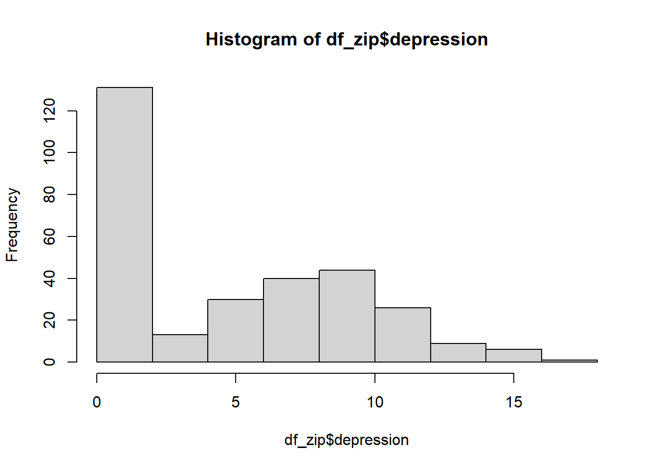
An ordinary normal mixture could attempt to approximate this distribution by estimating one Gaussian component with a very low mean and variance. But if our substantive hypothesis is specifically that one component represents structural zeros, we can encode that hypothesis directly.
For the first class, depression is fixed at zero. Because everyone represented by this component is assumed to have a depression score of zero, both its mean and variance are fixed to zero.
Smoking, however, is still allowed to vary normally in this class.
For the second class, depression has an estimated mean and variance. Smoking is regressed on depression, allowing us to estimate the association between depressive symptoms and smoking among individuals belonging to this continuous component.
model_zero <- "
  # Depression is a structural zero
  depression ~ 0*1
  depression ~~ 0*depression

  # Smoking remains normally distributed
  smoking ~ smoke_mean1*1
  smoking ~~ smoke_var1*smoking
"

model_depressed <- "
  # Continuous depression distribution
  depression ~ dep_mean*1
  depression ~~ dep_var*depression

  # Smoking depends on depression
  smoking ~ smoke_mean2*1
  smoking ~ b*depression
  smoking ~~ smoke_var2*smoking
"

fit_zip <- mx_mixture(
  model = list(
    model_zero,
    model_depressed
  ),
  data = df_zip
)
table_fit(fit_zip)| Minus2LogLikelihood | n | Parameters | observedStatistics | df | RMSEASquared | RMSEANull | modelName | AIC | BIC | saBIC | Classes | Entropy | prob_min | prob_max | n_min | n_max | LL |
|---|---|---|---|---|---|---|---|---|---|---|---|---|---|---|---|---|---|
| 2844.468 | 300 | 8 | 600 | 592 | 0 | 0.05 | mix2 | 2860.468 | 2890.098 | 2864.727 | 2 | 0.9111211 | 0.9791151 | 0.98411 | 0.4433333 | 0.5566667 | -1422.234 |
| label | est_sig | se | pval | confint | class |
|---|---|---|---|---|---|
| Means.smoking.class1 | 4.98*** | 0.18 | 0.00 | [4.63, 5.33] | class1 |
| Variances.depression.class1 | 1.98 | NA | NA | NA | class1 |
| Variances.smoking.class1 | 4.03*** | 0.51 | 0.00 | [3.03, 5.02] | class1 |
| Regressions.smoking.ON.depression.class2 | 0.11 | 0.06 | 0.05 | [-0.00, 0.22] | class2 |
| Means.smoking.class2 | 5.42*** | 0.50 | 0.00 | [4.45, 6.39] | class2 |
| Means.depression.class2 | 8.14*** | 0.25 | 0.00 | [7.64, 8.64] | class2 |
| Variances.smoking.class2 | 4.10*** | 0.46 | 0.00 | [3.20, 5.00] | class2 |
| Variances.depression.class2 | 8.93*** | 1.17 | 0.00 | [6.64, 11.21] | class2 |
| mix2.weights[1,1].NA | 1.00 | NA | NA | NA | NA |
| mix2.weights[1,2].NA | 1.25*** | 0.15 | 0.00 | [0.95, 1.55] | NA |
Note that the regression coefficient is estimated quite precisely.
5.5.3 Why not simply use mx_profiles()?
A conventional call such as
| label | est_sig | se | pval | confint | class |
|---|---|---|---|---|---|
| Regressions.smoking.ON.depression.class1 | -88175604.40 | NA | NA | NA | class1 |
| Means.smoking.class1 | 4.95 | 7.60 | 0.51 | [-9.95, 19.85] | class1 |
| Means.depression.class1 | -0.00 | 8278.93 | 1.00 | [-16226.40, 16226.40] | class1 |
| Variances.smoking.class1 | 4.04 | NA | NA | NA | class1 |
| Variances.depression.class1 | 0.00 | 6936309.37 | 1.00 | [-13594916.55, 13594916.55] | class1 |
| Regressions.smoking.ON.depression.class2 | 0.10 | 111.27 | 1.00 | [-217.98, 218.19] | class2 |
| Means.smoking.class2 | 5.46 | 12.93 | 0.67 | [-19.87, 30.80] | class2 |
| Means.depression.class2 | 8.08 | 8.75 | 0.36 | [-9.06, 25.23] | class2 |
| Variances.smoking.class2 | 4.07 | 4.53 | 0.37 | [-4.81, 12.95] | class2 |
| Variances.depression.class2 | 8.89*** | 2.07 | 0.00 | [4.83, 12.95] | class2 |
| mix2.weights[1,1].NA | 1.00 | NA | NA | NA | NA |
| mix2.weights[1,2].NA | 1.30 | 13.17 | 0.92 | [-24.52, 27.13] | NA |
Notice that this model returns nonsense coefficients.
5.6 Using OpenMx Models
The third interface to mx_mixture() is to supply a list of OpenMx::mxModel() objects.
This interface gives the user direct access to OpenMx matrices, algebra, constraints, and fit functions. It is the most flexible option, but it also requires substantially more knowledge of OpenMx.
Use this approach when the desired model cannot be expressed adequately using the lavaan-style syntax handled by as_ram().
5.7 Building models without immediately estimating them
By default, mx_mixture() estimates the model. Internally, run = TRUE causes tidySEM to obtain mixture starting values and run the OpenMx model.
During model development, it can be useful to create the model first without estimating it:
MxModel 'mix2'
type : default
$matrices : 'weights'
$algebras : NULL
$penalties : NULL
$constraints : NULL
$intervals : NULL
$latentVars : none
$manifestVars : none
$data : 150 x 2
$data means : NA
$data type: 'raw'
$submodels : 'class1' and 'class2'
$expectation : MxExpectationMixture
$fitfunction : MxFitFunctionML
$compute : NULL
$independent : FALSE
$options :
$output : FALSE
This allows advanced users to inspect or modify the generated OpenMx model before estimation.
These models typically contain the following matrices:
The ‘A’ argument refers to the A or asymmetric matrix in the RAM approach. This matrix consists of all of the asymmetric paths (one-headed arrows) in the model. A free parameter in any row and column describes a regression of the variable represented by that row regressed on the variable represented in that column.
The ‘S’ argument refers to the S or symmetric matrix in the RAM approach, and as such must be square. This matrix consists of all of the symmetric paths (two-headed arrows) in the model. A free parameter in any row and column describes a covariance between the variable represented by that row and the variable represented by that column. Variances are covariances between any variable at itself, which occur on the diagonal of the specified matrix.
The ‘F’ argument refers to the F or filter matrix in the RAM approach. If no latent variables are included in the model (i.e., the A and S matrices are of both of the same dimension as the data matrix), then the ‘F’ should refer to an identity matrix. If latent variables are included (i.e., the A and S matrices are not of the same dimension as the data matrix), then the ‘F’ argument should consist of a horizontal adhesion of an identity matrix and a matrix of zeros.
The ‘M’ argument refers to the M or means matrix in the RAM approach. It is a 1 x n matrix, where n is the number of manifest variables + the number of latent variables. The M matrix must be specified if either the mxData type is “cov” or “cor” and a means vector is provided, or if the mxData type is “raw”. Otherwise the M matrix is ignored.
You can access them as follows:
Each has several properties, including (starting) value, whether it is freely estimated or not, upper/lower bounds, labels, each of which you could modify by hand:
Once the specification is satisfactory, the model can be estimated using tidySEM’s OpenMx workflow.
5.8 Conclusion
mx_mixture() is the general-purpose mixture-modeling function underlying much of tidySEM’s OpenMx mixture functionality. It accepts a single dynamic model specification, class-specific syntax, or fully specified OpenMx models.
Use mx_mixture() when the scientific hypothesis concerns something that the standard wrappers do not expose directly: class-specific regression coefficients, particular equality constraints, or entirely different models between classes.