1 Introduction to Latent Class Analysis
This vignette covers the core ideas behind LCA, and takes you through the estimation of models with continuous, ordinal, and dichotomous indicators, and combinations of these. We focus on the practical decisions researchers face: evaluating model fit, assessing classification accuracy, interpreting model parameters, and reporting results clearly with publication-ready tables and figures.
To follow along and run the code yourself, open the file lca_introduction.qmd in the lca_course project, as explained in Appendix A.
After this vignette, you should be able to:
- Prepare a dataset for LCA
- fit latent profile models with continuous indicators using
mx_profiles(); - fit latent class models with ordinal or dichotomous indicators using
mx_lca(); - fit models that combine indicator types using
mx_mixed_lca(); - compare candidate class solutions using
table_fit(); - assess classification uncertainty using
class_prob(); - interpret class-specific parameters using
table_results(); - produce reporting-quality tables and figures
Note that this vignette roughly follows the steps outlines in the SMART-LCA Checklist (Standards for More Accuracy in Reporting of different Types of Latent Class Analysis), but not in detail. You can examine the checklist by running vignette("SMART_LCA_checklist", package = "tidySEM").
1.1 Pre-Analysis
In this case, we’re LCAs as toy examples to become familiar with the technique. This application of LCA is purely exploratory (there is no theory about the number and kind of classes). We are unsure if the indicators are valid and reliable for LCA, and our sample size is predetermined by the data available for secondary analysis. We will use data from the following paper:
Zhao K, Zhao Y, Xu W. Relationship between middle school students’ academic stress and physical exercise behavior from the perspective of Self-Determination Theory: The chained mediation of motivation and intention. PLoS One. 2025 Jan 3;20(1):e0316599. doi: 10.1371/journal.pone.0316599. PMID: 39752352; PMCID: PMC11698333.
These data are available in the file pone.0316599.s002.xlsx, and we can load them as follows:
Run View(df) to inspect the data.
1.1.1 Using Your Own Data
If you are using your own data, you might be able to load them by using or modifying one of the following functions:
1.2 Examining Observed Data
Scroll through the dataset; note that the bottom rows are all empty. We can drop them as follows:
Now, inspect descriptive statistics for the variables in the dataset. This is an important initial data-screening step because it helps us understand the structure of the data and identify features such as variable ranges, means, standard deviations, missing values, and the number of unique observed values.
| name | type | n | missing | unique | mean | median | mode | mode_value | sd | v | min | max | range | skew | skew_2se | kurt | kurt_2se |
|---|---|---|---|---|---|---|---|---|---|---|---|---|---|---|---|---|---|
| Grade | numeric | 290 | 0 | 3 | 2.044828 | 2 | 2 | NA | 0.9044627 | NA | 1 | 3 | 2 | -0.0886256 | -0.3096579 | -1.7774984 | -3.1157225 |
| Age | numeric | 290 | 0 | 4 | 13.758621 | 14 | 14 | NA | 0.9577646 | NA | 12 | 15 | 3 | -0.1663658 | -0.5812821 | -1.0000580 | -1.7529711 |
| Gender | numeric | 290 | 0 | 2 | 1.600000 | 2 | 2 | NA | 0.4907448 | NA | 1 | 2 | 1 | -0.4103740 | -1.4338470 | -1.8443610 | -3.2329238 |
| TS1 | numeric | 290 | 0 | 7 | 2.944828 | 3 | 3 | NA | 1.5464182 | NA | 1 | 7 | 6 | 0.3584376 | 1.2523814 | -0.6547142 | -1.1476285 |
| TS2 | numeric | 290 | 0 | 7 | 3.110345 | 3 | 3 | NA | 1.5479297 | NA | 1 | 7 | 6 | 0.3272700 | 1.1434818 | -0.6096701 | -1.0686720 |
| TS3 | numeric | 290 | 0 | 7 | 2.541379 | 2 | 2 | NA | 1.6130989 | NA | 1 | 7 | 6 | 0.8463815 | 2.9572575 | -0.1107475 | -0.1941259 |
| TS4 | numeric | 290 | 0 | 7 | 2.962069 | 3 | 3 | NA | 1.4535278 | NA | 1 | 7 | 6 | 0.2025191 | 0.7076019 | -0.7640309 | -1.3392464 |
| SOS1 | numeric | 290 | 0 | 7 | 4.624138 | 5 | 5 | NA | 1.6762446 | NA | 1 | 7 | 6 | -0.3195548 | -1.1165248 | -0.7110256 | -1.2463349 |
| SOS2 | numeric | 290 | 0 | 7 | 3.468965 | 3 | 3 | NA | 1.7805375 | NA | 1 | 7 | 6 | 0.3438411 | 1.2013811 | -0.7846706 | -1.3754251 |
| SOS3 | numeric | 290 | 0 | 7 | 2.724138 | 2 | 2 | NA | 1.8168102 | NA | 1 | 7 | 6 | 0.9002934 | 3.1456257 | -0.2517256 | -0.4412420 |
| SOS4 | numeric | 290 | 0 | 7 | 2.920690 | 3 | 3 | NA | 1.4754928 | NA | 1 | 7 | 6 | 0.4304447 | 1.5039743 | -0.5976676 | -1.0476332 |
| PS1 | numeric | 290 | 0 | 7 | 4.603448 | 5 | 5 | NA | 1.6568998 | NA | 1 | 7 | 6 | -0.3071955 | -1.0733413 | -0.5118607 | -0.8972250 |
| PS2 | numeric | 290 | 0 | 7 | 2.627586 | 2 | 2 | NA | 1.5934330 | NA | 1 | 7 | 6 | 0.7964309 | 2.7827304 | -0.1185252 | -0.2077592 |
| PS3 | numeric | 290 | 0 | 7 | 3.189655 | 3 | 3 | NA | 1.6993475 | NA | 1 | 7 | 6 | 0.2628300 | 0.9183282 | -1.0590921 | -1.8564500 |
| PS4 | numeric | 290 | 0 | 7 | 3.351724 | 3 | 3 | NA | 1.8546902 | NA | 1 | 7 | 6 | 0.2754714 | 0.9624973 | -1.0364063 | -1.8166848 |
| PS5 | numeric | 290 | 0 | 7 | 3.048276 | 3 | 3 | NA | 1.7522345 | NA | 1 | 7 | 6 | 0.4504039 | 1.5737115 | -0.8333342 | -1.4607260 |
| AM1 | numeric | 290 | 0 | 7 | 4.431034 | 4 | 4 | NA | 1.5261512 | NA | 1 | 7 | 6 | -0.3711418 | -1.2967696 | -0.0725992 | -0.1272570 |
| AM2 | numeric | 290 | 0 | 7 | 4.806897 | 5 | 5 | NA | 1.4637325 | NA | 1 | 7 | 6 | -0.5346357 | -1.8680175 | 0.1543142 | 0.2704926 |
| AM3 | numeric | 290 | 0 | 7 | 4.603448 | 4 | 4 | NA | 1.4757516 | NA | 1 | 7 | 6 | -0.3145517 | -1.0990438 | -0.0388020 | -0.0680148 |
| AM4 | numeric | 290 | 0 | 7 | 4.500000 | 4 | 4 | NA | 1.4676441 | NA | 1 | 7 | 6 | -0.2149216 | -0.7509362 | -0.0517850 | -0.0907723 |
| AM5 | numeric | 290 | 0 | 7 | 4.713793 | 5 | 5 | NA | 1.4918983 | NA | 1 | 7 | 6 | -0.4510817 | -1.5760798 | 0.0241397 | 0.0423138 |
| CM1 | numeric | 290 | 0 | 7 | 2.889655 | 3 | 3 | NA | 1.5002525 | NA | 1 | 7 | 6 | 0.6662803 | 2.3279840 | 0.1091563 | 0.1913368 |
| CM2 | numeric | 290 | 0 | 7 | 2.865517 | 3 | 3 | NA | 1.4381784 | NA | 1 | 7 | 6 | 0.3500659 | 1.2231304 | -0.4922577 | -0.8628634 |
| CM3 | numeric | 290 | 0 | 7 | 3.306897 | 4 | 4 | NA | 1.5559754 | NA | 1 | 7 | 6 | 0.2778648 | 0.9708599 | -0.3504062 | -0.6142163 |
| CM4 | numeric | 290 | 0 | 7 | 3.427586 | 4 | 4 | NA | 1.6290818 | NA | 1 | 7 | 6 | 0.3380570 | 1.1811716 | -0.3672153 | -0.6436804 |
| BI1 | numeric | 290 | 0 | 7 | 4.782759 | 5 | 5 | NA | 1.4376473 | NA | 1 | 7 | 6 | -0.4300435 | -1.5025725 | 0.1265571 | 0.2218381 |
| BI2 | numeric | 290 | 0 | 7 | 4.913793 | 5 | 5 | NA | 1.3680042 | NA | 1 | 7 | 6 | -0.6191560 | -2.1633314 | 0.5172608 | 0.9066907 |
| BI3 | numeric | 290 | 0 | 7 | 4.982759 | 5 | 5 | NA | 1.4128841 | NA | 1 | 7 | 6 | -0.6660460 | -2.3271653 | 0.5313738 | 0.9314289 |
| BH1 | numeric | 290 | 0 | 7 | 4.986207 | 5 | 5 | NA | 1.7068403 | NA | 1 | 7 | 6 | -0.4282368 | -1.4962598 | -0.6824016 | -1.1961608 |
| BH2 | numeric | 290 | 0 | 7 | 3.465517 | 3 | 3 | NA | 1.5341050 | NA | 1 | 7 | 6 | 0.6271490 | 2.1912593 | 0.0702681 | 0.1231707 |
The type column tells you the measurement level of each variable. The tidySEM package supports latent class analysis with numeric (or integer) and ordered variables.
Numeric and integer variables should be truly continuous (e.g., centimeters), or you must be willing to assume that they behave as continuous (scale mean scores in a questionnaire).
Ordinal indicators consist of categories that have a meaningful order, such as Likert responses ranging from strongly disagree to strongly agree.
Note that integer variables containing only a small number of values could be numeric score, but could also be ordered. The correct treatment depends on what the numbers mean, not merely on how R stores them. Check the unique column of descriptives() to see how many unique values there are; this may alert you to such issues.
If you have variables with other data types than numeric/integer/ordered - you will need to convert them.
One key issue is that variables are not always correctly stored. The type column may not correspond to the variable’s substantive measurement level. For example, you might have a variable of type integer with values 1, 2, but which actually represents employment, with values Unemployed and Employed. Moreover, an integer variable may represent a truly continuous quantity (e.g., number of children), or an ordinal Likert scale, in which case it should be recoded to ordered. Similarly, a factor may represent an unordered categorical variable with several categories. For LCA, each category should be coded as a binary ordered variable.
You should therefore inspect both the variable type and the meaning of the variable before deciding how it should enter the model.
Quiz
An integer variable with values (1,2), which represent Employed and Unemployed, should be recoded to factor.
An ordinal Likert scale should be coded as a numeric variable.
The factor variable 'major in university', with four different values, should be coded as four binary variables of type ordered for LCA.
1.3 Data Preprocessing
If a variable is incorrectly coded, you may be able to restore its correct type. Here are a few examples of type conversions:
[1] "character"[1] 5.1 4.9 4.7 NA 5.0 5.4[1] "integer"[1] 2 3 2 5 3 4
Levels: 2 < 3 < 4 < 5[1] "factor"| Humanities | Medicine | Social.science |
|---|---|---|
| 0 | 1 | 0 |
| 1 | 0 | 0 |
| 1 | 0 | 0 |
| 0 | 1 | 0 |
| 0 | 0 | 1 |
| 0 | 1 | 0 |
The final command takes an unordered factor and represents it as a set of binary dummy variables; one for each category. These dummy variables can then be added to the analysis dataset.
Note that, in our example dataset, all variable types are numeric, even though some must be integer (age), and others must be factors (Gender) or ordered (all Likert scales). Note that all variables have just few low number of unique values; this is another hint that some recoding is in order.
Here we recode ‘gender’ from its original numeric codes into a factor variable. We also attach meaningful text labels to the numeric categories so that subsequent tables and output are easier to understand. The ‘levels’ argument specifies the original codes found in the dataset, while ‘labels’ specifies the corresponding category names that R should display instead.
Several variables in the dataset are individual questionnaire items that belong to broader multi-item scales.
We can use these to practice two things:
- Computing numeric scale mean scores
- Encoding them as ordered variables
We will compute the scale scores first, because this still requires these variables to be numeric.
For example, the scale named TS consists of TS1 through TS4, while SOS consists of SOS1 through SOS4. I like to store this information in a list, as this would allow you to, for example, easily perform psychometric analyses for every scale automatically (which is out of scope for the current tutorial).
# To prepare the scales list, I used:
scales_list <- grep("\\w{2}\\d", names(df), value = TRUE)
scalenames <- unique(gsub("\\d", "", scales_list))
scales_list <- lapply(scalenames, grep, x = names(df), value = TRUE)
names(scales_list) <- scalenames

# This gives the list below; you can also construct it for your dataset by hand:
scales_list <- list(
  TS = c("TS1", "TS2", "TS3", "TS4"),
  SOS = c("SOS1", "SOS2", "SOS3", "SOS4"),
  PS = c("PS1", "PS2", "PS3", "PS4", "PS5"),
  AM = c("AM1", "AM2", "AM3", "AM4", "AM5"),
  CM = c("CM1", "CM2", "CM3", "CM4"),
  BI = c("BI1", "BI2", "BI3"),
  BH = c("BH1", "BH2")
  )
To compute mean scale scores, we can use:
Second, the encode these items as ordered variables, we could grab all relevant variables based on the naming pattern (these variable names end with a number), or we can take all items in the scales_list using unlist():
 [1] "TS1"  "TS2"  "TS3"  "TS4"  "SOS1" "SOS2" "SOS3" "SOS4" "PS1"  "PS2"
[11] "PS3"  "PS4"  "PS5"  "AM1"  "AM2"  "AM3"  "AM4"  "AM5"  "CM1"  "CM2"
[21] "CM3" "CM4" "BI1" "BI2" "BI3" "BH1" "BH2" Then, we can recode these variables as ordered:
Inspect the cleaned dataset again before fitting the model. Check that numeric indicators really represent continuous quantities, ordered indicators have the intended category order, and binary indicators contain exactly two possible response categories. Also check for unexpected values, unused factor levels, miscoded missing values, and variables with little or no variation.
1.4 Missing Data
This dataset has no missing data. However, you can increase the challenge for yourself by adding some missingness. If you want to do this - do it immediately after loading the data and removing the empty rows, with code like this:
Regardless of the presence of missingness or not, tidySEM uses FIML which includes cases with partially missing data.
1.5 Model Specification
The type of model you can specify depends partially on the measurement level of your indicators:
| Indicator type | Typical examples | tidySEM function | Class-specific quantities |
|---|---|---|---|
| Continuous | test scores, reaction time, symptom sum scores | mx_profiles() |
means, variances, possibly covariances |
| Ordinal | Likert items, ordered severity categories | mx_lca() |
category probabilities / thresholds |
| Dichotomous | yes/no, present/absent, correct/incorrect | mx_lca() |
response probabilities |
| Mixed | a combination of the above | mx_mixed_lca() |
parameters appropriate to each indicator type |
Quiz
A dataset containing three mean scale score variables would be analyzed with:
A dataset containing ten ordinal questionnaire items would be analyzed with:
A dataset containing both continuous scale scores and binary indicators would require:
1.6 Latent Profile Analysis (LPA) with Continuous Indicators
We will use two scale scores from the Zhao dataset as a teaching example; specifically, c("AM", "CM"), which represent autonomous and controlled motivation. You can increase the challenge level of this tutorial by using your own dataset, or by selecting different scales. For example, c("TS", "SOS", "PS"), which represent three sources of stress/pressure: teacher stress, social stress, and parent stress.
Note that standardizing indicators is not required and should not affect results, with two caveats: if continuous indicators are on very different scales (e.g., the variance differs by a factor 10+), this can cause problems for model convergence. Second, this can make plots harder to read because the plotting range of one variable could be much smaller than another.
1.6.1 Model Specification
The arguments variances and covariances control the model specification for LPA. For example, a model with equal variances and zero covariances assumpes that every indicator has the same residual variance across classes, and that indicators are “locally independent” (=uncorrelated) within each class, even if they should be correlated at the sample level. Note that you can also specify different (co)variance structures, either for thorough exploration of because you have some theory about e.g., smaller variance in some classes, or different correlations between classes. See the help file by running ?mx_profiles. For example, you could specify the code below.
Note that this analysis will take a very long time because these are many models and some of them are hard to estimate. For any computationally intensive analyses like this, we can save the results to a file, so you can load the results from that file directly without having to wait for the code to run. We do recommend that you experiment with running some analyses yourself, of course.
| Name | Classes | LL | n | Parameters | AIC | BIC | saBIC | Entropy | prob_min | prob_max | n_min | n_max | warning | np_ratio | np_local |
|---|---|---|---|---|---|---|---|---|---|---|---|---|---|---|---|
| equal var 1 | 1.00 | -938.90 | 290.00 | 4 | 1885.79 | 1900.47 | 1887.79 | 1.00 | 1.00 | 1.00 | 1.00 | 1.00 | NA | 72.50 | 72.50 |
| equal var 2 | 2.00 | -915.49 | 290.00 | 7 | 1844.99 | 1870.68 | 1848.48 | 0.70 | 0.69 | 0.97 | 0.15 | 0.85 | NA | 41.43 | 14.67 |
| equal var 3 | 3.00 | -894.71 | 290.00 | 10 | 1809.41 | 1846.11 | 1814.40 | 0.82 | 0.87 | 0.95 | 0.10 | 0.61 | NA | 29.00 | 10.50 |
| equal var 4 | 4.00 | -888.40 | 290.00 | 13 | 1802.80 | 1850.51 | 1809.28 | 0.85 | 0.80 | 0.95 | 0.05 | 0.58 | NA | 22.31 | 6.00 |
| equal var 5 | 5.00 | -885.87 | 290.00 | 16 | 1803.74 | 1862.46 | 1811.72 | 0.82 | 0.48 | 0.96 | 0.03 | 0.58 | NA | 18.12 | 3.75 |
| free var, equal cov 1 | 1.00 | -913.54 | 290.00 | 5 | 1837.07 | 1855.42 | 1839.57 | 1.00 | 1.00 | 1.00 | 1.00 | 1.00 | NA | 58.00 | 58.00 |
| free var, equal cov 2 | 2.00 | -904.62 | 290.00 | 10 | 1829.23 | 1865.93 | 1834.22 | 0.29 | 0.51 | 0.91 | 0.24 | 0.76 | NA | 29.00 | 15.56 |
| free var, equal cov 3 | 3.00 | -794.43 | 290.00 | 15 | 1618.85 | 1673.90 | 1626.33 | 0.79 | 0.77 | 1.00 | 0.16 | 0.60 | TRUE | 19.33 | 10.85 |
| free var, equal cov 4 | 4.00 | -754.85 | 290.00 | 20 | 1549.70 | 1623.10 | 1559.67 | 0.83 | 0.84 | 1.00 | 0.08 | 0.38 | TRUE | 14.50 | 5.41 |
| free var, equal cov 5 | 5.00 | -828.60 | 290.00 | 25 | 1707.19 | 1798.94 | 1719.66 | 0.86 | 0.80 | 0.97 | 0.02 | 0.44 | TRUE | 11.60 | 1.43 |
More complex models are not automatically better: extra parameters can create unstable solutions, tiny classes, or local maxima. Think about which models make sense to estimate, and how many classes your data could reasonably support.
1.6.2 Maximum Number of Classes
We can set an upper limit on the number of classes to estimate, for example, by saying we want to aim for 20 observations per parameter, if cases would be evenly split between classes. We could then estimate 290/20 = 14.5 parameters. With 2 indicators, zero covariances, and equal variances, the number of parameters for our model is:
- k-1 mixture weights
- k*2 means
- 2 variances
Which would give this many cases per parameter:
 [1] 72.500000 41.428571 29.000000 22.307692 18.125000 15.263158 13.181818
 [8] 11.600000 10.357143  9.354839
So we could estimate at least 4 classes. Let’s round up and estimate 1:5 class solutions:
1.6.3 Class Enumeration
First, extract a model fit table:
| Name | Classes | LL | n | Parameters | AIC | BIC | saBIC | Entropy | prob_min | prob_max | n_min | n_max | np_ratio | np_local |
|---|---|---|---|---|---|---|---|---|---|---|---|---|---|---|
| equal var 1 | 1 | -938.8958 | 290 | 4 | 1885.792 | 1900.471 | 1887.786 | 1.0000000 | 1.0000000 | 1.0000000 | 1.0000000 | 1.0000000 | 72.50000 | 72.50000 |
| equal var 2 | 2 | -915.4934 | 290 | 7 | 1844.987 | 1870.676 | 1848.478 | 0.6995815 | 0.6881145 | 0.9677946 | 0.1517241 | 0.8482759 | 41.42857 | 14.66667 |
| equal var 3 | 3 | -894.7056 | 290 | 10 | 1809.411 | 1846.110 | 1814.398 | 0.8159663 | 0.8741811 | 0.9504706 | 0.0965517 | 0.6137931 | 29.00000 | 10.50000 |
| equal var 4 | 4 | -892.8343 | 290 | 13 | 1811.669 | 1859.377 | 1818.152 | 0.7966132 | 0.3619379 | 0.9541764 | 0.0206897 | 0.6137931 | 22.30769 | 2.40000 |
| equal var 5 | 5 | -885.8717 | 290 | 16 | 1803.743 | 1862.462 | 1811.723 | 0.8231484 | 0.4849168 | 0.9562938 | 0.0310345 | 0.5793103 | 18.12500 | 3.75000 |
1.6.3.1 BIC
One well-supported criterion for class enumeration is the BIC: a relative fit index that rewards good fit and penalizes model complexity. The absolute BIC value has no substantive meaning; you can compare BIC values of models fitted to the same data, and lower values are preferred. We can see that the three-class model has the lowest BIC:
1.6.3.2 BLRT
We can also conduct a bootstrapped likelihood ratio test, which asks whether a model with \(k\) classes improves fit over a model with \(k-1\) classes. However, this test is extremely computationally expensive. Before we do so, it is useful to check if we can eliminate some models from consideration (also see next section). For example, note that np_local, the minimum number of cases assigned to a class divided by the number of parameters in that class, is as low as 2.4 for models with 4-5 classes. You want a healthy number of cases per parameter, so we can exclude these two models, then perform our BLRT:
| null | alt | lr | df | blrt_p | samples | |
|---|---|---|---|---|---|---|
| equal var 1 | mix1 | mix2 | 46.80472 | 3 | 0 | 100 |
| equal var 2 | mix2 | mix3 | 41.57568 | 3 | 0 | 98 |
We see that adding classes leads to a significant improvement in model fit.
1.6.4 Eliminating Models from Consideration
As mentioned before, we will eliminate the 4-5 class models because they have a very low number of observations per parameter.
We can also check for any model convergence problems; a value other than 0 for the convergence status can indicate a problem:
equal var 1 equal var 2 equal var 3 equal var 4 equal var 5
          0           0           0           0           0
Another consideration is that classification diagnostics are poor for the 4-5 class models:
| Entropy | prob_min | prob_max |
|---|---|---|
| 1.0000000 | 1.0000000 | 1.0000000 |
| 0.6995815 | 0.6881145 | 0.9677946 |
| 0.8159663 | 0.8741811 | 0.9504706 |
| 0.7966132 | 0.3619379 | 0.9541764 |
| 0.8231484 | 0.4849168 | 0.9562938 |
The entropy statistic is an overall summary of class separation, where values approaching 1 indicate clear delineation of classes (Celeux & Soromenho, 1996).
The statistics prob_min and prob_max give us the minumum and maximum of the diagonal of the mostlikely.class classification table (see ?class_prob). If C is the true class of an observation, and N is the most likely class based on the model, then this table shows the probability P(N==i|C==j). The diagonal represents the probability that observations in each class will be correctly classified. We see that prob_min is very low for the 4-5 class models; thus, for some classes, there is a low probability that its members will be correctly classified. This is also reflected in the entropy.
1.6.5 Reporting Results
We already obtained the model fit table. There are many ways to prepare it for a scientific paper. The regular formatting function in R has some peculiar behavior; it does not guarantee that a certain number of decimals are displayed. This is a design choice in R, and has to do with the principle of “significant figures”. However, APA style simply requires reporting to double digits. So let’s consider two options:
| Name | Classes | LL | n | Parameters | AIC | BIC | saBIC | Entropy | prob_min | prob_max | n_min | n_max | np_ratio | np_local |
|---|---|---|---|---|---|---|---|---|---|---|---|---|---|---|
| equal var 1 | 1 | -939 | 290 | 4 | 1886 | 1900 | 1888 | 1.00 | 1.00 | 1.00 | 1.000 | 1.00 | 72 | 72.5 |
| equal var 2 | 2 | -915 | 290 | 7 | 1845 | 1871 | 1848 | 0.70 | 0.69 | 0.97 | 0.152 | 0.85 | 41 | 14.7 |
| equal var 3 | 3 | -895 | 290 | 10 | 1809 | 1846 | 1814 | 0.82 | 0.87 | 0.95 | 0.097 | 0.61 | 29 | 10.5 |
| equal var 4 | 4 | -893 | 290 | 13 | 1812 | 1859 | 1818 | 0.80 | 0.36 | 0.95 | 0.021 | 0.61 | 22 | 2.4 |
| equal var 5 | 5 | -886 | 290 | 16 | 1804 | 1862 | 1812 | 0.82 | 0.48 | 0.96 | 0.031 | 0.58 | 18 | 3.8 |
Based on the BIC, the elimination of the 4-5 class models, and significant BLRT tests, we would retain a 3-class model.
The class proportions of this model are:
$sum.posterior
   class     count proportion
1 class1 171.83359  0.5925296
2 class2  88.42000  0.3048965
3 class3  29.74641  0.1025738
We can examine the parameters of this model as follows:
| label | est_sig | se | pval | confint | class |
|---|---|---|---|---|---|
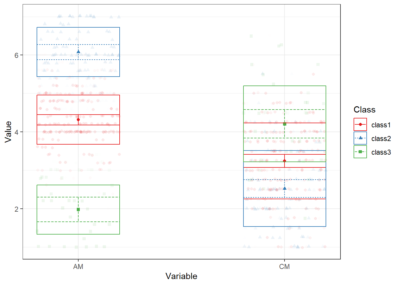
| Means.AM.class1 | 4.31*** | 0.07 | 0.00 | [4.18, 4.45] | class1 |
| Means.CM.class1 | 3.24*** | 0.09 | 0.00 | [3.07, 3.41] | class1 |
| Variances.AM.class1 | 0.41*** | 0.05 | 0.00 | [0.32, 0.51] | class1 |
| Variances.CM.class1 | 0.98*** | 0.09 | 0.00 | [0.81, 1.14] | class1 |
| Means.AM.class2 | 6.08*** | 0.10 | 0.00 | [5.88, 6.27] | class2 |
| Means.CM.class2 | 2.52*** | 0.12 | 0.00 | [2.29, 2.76] | class2 |
| Means.AM.class3 | 1.98*** | 0.17 | 0.00 | [1.65, 2.30] | class3 |
| Means.CM.class3 | 4.20*** | 0.19 | 0.00 | [3.83, 4.57] | class3 |
| mix3.weights[1,1].NA | 1.00 | NA | NA | NA | NA |
| mix3.weights[1,2].NA | 0.51*** | 0.09 | 0.00 | [0.34, 0.69] | NA |
| mix3.weights[1,3].NA | 0.17*** | 0.04 | 0.00 | [0.09, 0.25] | NA |
Notice that we get one estimate for the variances (because these are equal across classes), no covariances, and unique estimates for the means across classes.
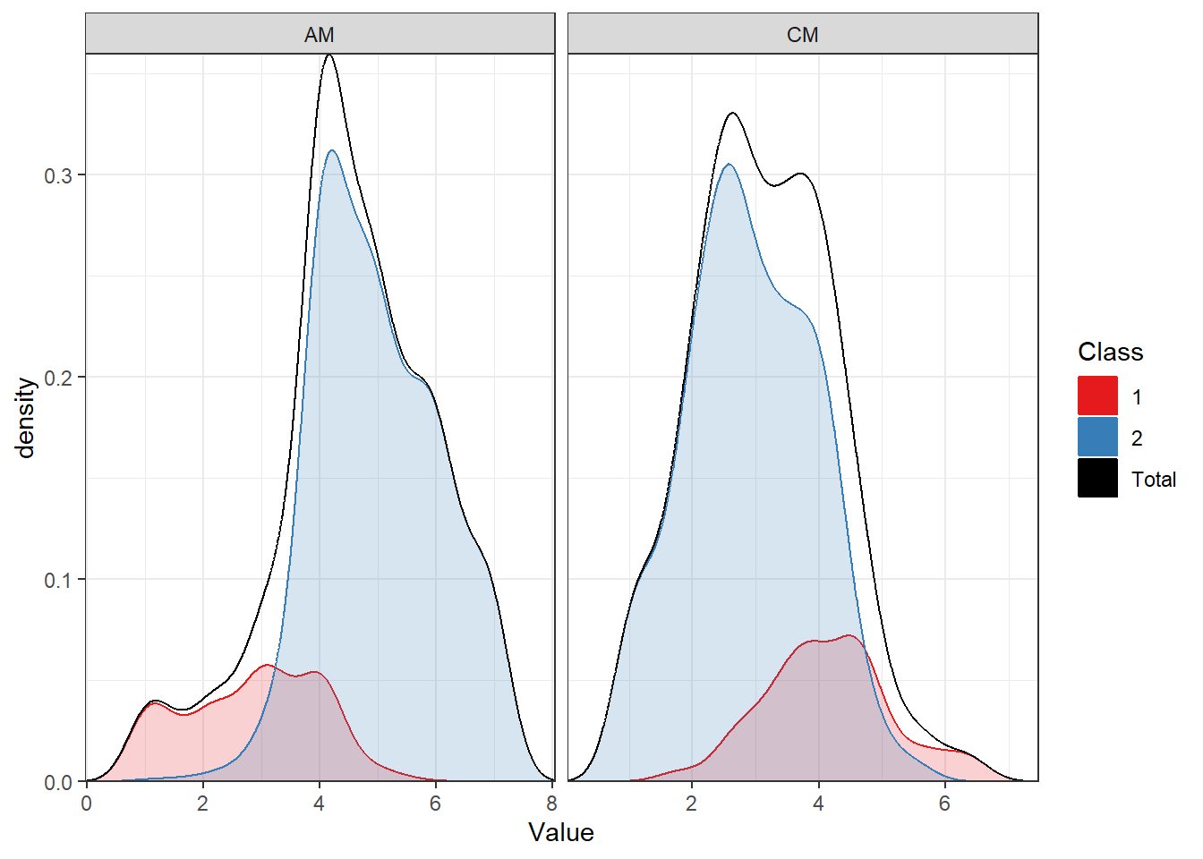
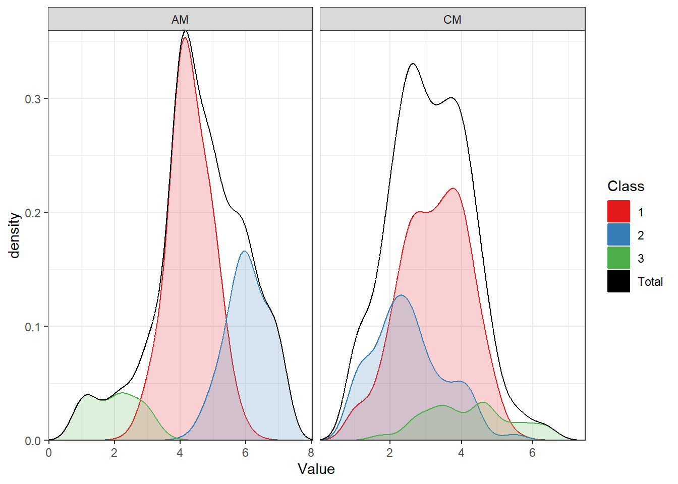
The pattern of results is easier to see when plotting it:
Quiz
Which class has moderate values on both indicators?
Class 2 has a high mean for both AM and CM
The marginal (whole-sample) distribution of both variables is pretty close to normally distributed.
Based on these results (relatively low class separability and approximately normal distribution of indicators, we should seriously consider the possibility that there are no distinct classes.
1.7 Latent Class Analysis with Ordinal indicators
We can conduct ordinal LCA by using some of the raw items underlying the scale scores, for example:
For a model with ordinal indicators, there is (currently) only one parametrization available. Specifically, we represent each ordinal variable as a latent normal variable with thresholds representing the quantiles of people who score a particular score or lower. In these models, each variable will have a number of thresholds equal to the number of response options minus one. It is easy to see that this model will have more parameters than the LPA model. If L is the number of levels of our ordinal indicators, and M is the number of indicators:
- k-1 mixture weights
- k((L-1)M) thresholds
Since our indicators have 7 categories, this gives:
 [1] 16.111111  7.837838  5.178571  3.866667  3.085106  2.566372  2.196970
 [8]  1.920530  1.705882  1.534392
Note that even for a 1-class model, we have fewer than 20 observations per parameter. Thus, we might doubt whether we have enough data here to estimate more than one class. For educational purposes - we will proceed, but to save time estimating overly complex models, we omit the 4-5 class models.
| Name | Classes | LL | n | Parameters | AIC | BIC | saBIC | Entropy | prob_min | prob_max | n_min | n_max | np_ratio | np_local |
|---|---|---|---|---|---|---|---|---|---|---|---|---|---|---|
| 1 | 1 | -1485.423 | 290 | 18 | 3006.847 | 3072.905 | 3015.824 | 1.0000000 | 1.0000000 | 1.0000000 | 1.0000000 | 1.0000000 | 16.111111 | 16.111111 |
| 2 | 2 | -1313.780 | 290 | 37 | 2701.559 | 2837.345 | 2720.011 | 0.8707661 | 0.9542104 | 0.9690095 | 0.4931034 | 0.5068966 | 7.837838 | 7.944444 |
| 3 | 3 | -1230.037 | 290 | 56 | 2572.075 | 2777.588 | 2600.002 | 0.8956807 | 0.9513416 | 0.9666826 | 0.1586207 | 0.5103448 | 5.178571 | 2.555556 |
The BIC indicates that adding classes improves model fit. However, even for the 2-class model, the number of cases/parameters in the smallest class (np_local) is smaller than 10. Thus, we might be skeptical about selecting more than 1 class for these data. For educational purposes, however, let’s examine the 2-class solution.
| label | est_sig | se | pval | confint | class |
|---|---|---|---|---|---|
| Variances.AM1.class1 | 1.00 | NA | NA | NA | class1 |
| Variances.AM2.class1 | 1.00 | NA | NA | NA | class1 |
| Variances.AM3.class1 | 1.00 | NA | NA | NA | class1 |
| class1.Thresholds[1,1].class1 | -1.14*** | 0.13 | 0.00 | [-1.40, -0.88] | class1 |
| class1.Thresholds[1,2].class1 | -1.45*** | 0.15 | 0.00 | [-1.75, -1.15] | class1 |
| class1.Thresholds[1,3].class1 | -1.40*** | 0.15 | 0.00 | [-1.70, -1.11] | class1 |
| class1.Thresholds[2,1].class1 | -0.84*** | 0.12 | 0.00 | [-1.07, -0.60] | class1 |
| class1.Thresholds[2,2].class1 | -1.08*** | 0.13 | 0.00 | [-1.33, -0.82] | class1 |
| class1.Thresholds[2,3].class1 | -0.99*** | 0.13 | 0.00 | [-1.24, -0.75] | class1 |
| class1.Thresholds[3,1].class1 | -0.34** | 0.11 | 0.00 | [-0.56, -0.13] | class1 |
| class1.Thresholds[3,2].class1 | -0.64*** | 0.11 | 0.00 | [-0.87, -0.42] | class1 |
| class1.Thresholds[3,3].class1 | -0.52*** | 0.11 | 0.00 | [-0.74, -0.30] | class1 |
| class1.Thresholds[4,1].class1 | 1.53*** | 0.21 | 0.00 | [1.13, 1.94] | class1 |
| class1.Thresholds[4,2].class1 | 0.78*** | 0.14 | 0.00 | [0.49, 1.06] | class1 |
| class1.Thresholds[4,3].class1 | 1.29*** | 0.18 | 0.00 | [0.94, 1.65] | class1 |
| class1.Thresholds[5,1].class1 | 2.22*** | 0.36 | 0.00 | [1.53, 2.92] | class1 |
| class1.Thresholds[5,2].class1 | 1.58*** | 0.19 | 0.00 | [1.21, 1.95] | class1 |
| class1.Thresholds[5,3].class1 | 2.61*** | 0.58 | 0.00 | [1.47, 3.75] | class1 |
| class1.Thresholds[6,1].class1 | 2.47*** | 0.36 | 0.00 | [1.77, 3.17] | class1 |
| class1.Thresholds[6,2].class1 | 1.79*** | 0.20 | 0.00 | [1.40, 2.18] | class1 |
| class1.Thresholds[6,3].class1 | 2.61*** | 0.57 | 0.00 | [1.50, 3.73] | class1 |
| Variances.AM1.class2 | 1.00 | NA | NA | NA | class2 |
| Variances.AM2.class2 | 1.00 | NA | NA | NA | class2 |
| Variances.AM3.class2 | 1.00 | NA | NA | NA | class2 |
| class2.Thresholds[1,1].class2 | -165.71 | NA | NA | NA | class2 |
| class2.Thresholds[1,2].class2 | -12.90 | NA | NA | NA | class2 |
| class2.Thresholds[1,3].class2 | -300.65 | NA | NA | NA | class2 |
| class2.Thresholds[2,1].class2 | -162.99 | NA | NA | NA | class2 |
| class2.Thresholds[2,2].class2 | -10.43 | NA | NA | NA | class2 |
| class2.Thresholds[2,3].class2 | -13.60 | NA | NA | NA | class2 |
| class2.Thresholds[3,1].class2 | -2.14*** | 0.29 | 0.00 | [-2.71, -1.57] | class2 |
| class2.Thresholds[3,2].class2 | -8.33 | NA | NA | NA | class2 |
| class2.Thresholds[3,3].class2 | -2.45*** | 0.36 | 0.00 | [-3.17, -1.74] | class2 |
| class2.Thresholds[4,1].class2 | -1.04*** | 0.17 | 0.00 | [-1.37, -0.72] | class2 |
| class2.Thresholds[4,2].class2 | -1.88* | 0.87 | 0.03 | [-3.58, -0.18] | class2 |
| class2.Thresholds[4,3].class2 | -1.24*** | 0.18 | 0.00 | [-1.60, -0.88] | class2 |
| class2.Thresholds[5,1].class2 | -0.09 | 0.12 | 0.46 | [-0.31, 0.14] | class2 |
| class2.Thresholds[5,2].class2 | -0.37 | 0.84 | 0.66 | [-2.01, 1.27] | class2 |
| class2.Thresholds[5,3].class2 | -0.24 | 0.12 | 0.05 | [-0.48, 0.00] | class2 |
| class2.Thresholds[6,1].class2 | 0.95*** | 0.13 | 0.00 | [0.70, 1.20] | class2 |
| class2.Thresholds[6,2].class2 | 0.76 | 0.84 | 0.36 | [-0.88, 2.40] | class2 |
| class2.Thresholds[6,3].class2 | 0.74*** | 0.12 | 0.00 | [0.50, 0.98] | class2 |
| mix2.weights[1,1].NA | 1.00 | NA | NA | NA | NA |
| mix2.weights[1,2].NA | 0.94*** | 0.13 | 0.00 | [0.68, 1.20] | NA |
We see that all the parameters are thresholds (and a mixture weight).
These thresholds are z-values at which a standard normal distribution would be intersected so that the proportion of participants falling below the threshold corresponds to the proportion of particiants who selected that answer category or lower. We can plot this to give you an intuitive understanding, for example, for the thresholds for variable AM1 in class 1:
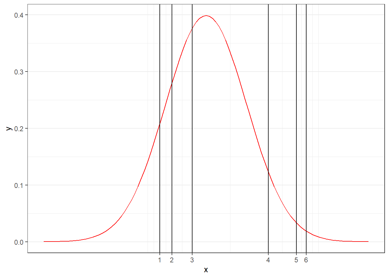
This figure implies that the most common response to AM1 in class 1 is 4, quite a few people score 1, and very few people score 6 or 7. We can do a sanity check to confirm this interpretation by assigning people to their most likely class (note that this ignores classification uncertainty), and then tabulating the observed scores of AM1 for the people who are assigned class 1:
 1  2  3  4  5  6  7
19 11 25 85  5  1  1
Another way to interpret the threshold parameters is to convert them to the estimated probability of choosing each response category:
| Variable | Category | Probability | group |
|---|---|---|---|
| AM1 | 1 | 0.13 | class1 |
| AM1 | 2 | 0.07 | class1 |
| AM1 | 3 | 0.17 | class1 |
| AM1 | 4 | 0.57 | class1 |
| AM1 | 5 | 0.05 | class1 |
| AM1 | 6 | 0.01 | class1 |
| AM1 | 7 | 0.01 | class1 |
| AM2 | 1 | 0.07 | class1 |
| AM2 | 2 | 0.07 | class1 |
| AM2 | 3 | 0.12 | class1 |
| AM2 | 4 | 0.52 | class1 |
| AM2 | 5 | 0.16 | class1 |
| AM2 | 6 | 0.02 | class1 |
| AM2 | 7 | 0.04 | class1 |
| AM3 | 1 | 0.08 | class1 |
| AM3 | 2 | 0.08 | class1 |
| AM3 | 3 | 0.14 | class1 |
| AM3 | 4 | 0.60 | class1 |
| AM3 | 5 | 0.09 | class1 |
| AM3 | 6 | 0.00 | class1 |
| AM3 | 7 | 0.00 | class1 |
| AM1 | 1 | 0.00 | class2 |
| AM1 | 2 | 0.00 | class2 |
| AM1 | 3 | 0.02 | class2 |
| AM1 | 4 | 0.13 | class2 |
| AM1 | 5 | 0.32 | class2 |
| AM1 | 6 | 0.36 | class2 |
| AM1 | 7 | 0.17 | class2 |
| AM2 | 1 | 0.00 | class2 |
| AM2 | 2 | 0.00 | class2 |
| AM2 | 3 | 0.00 | class2 |
| AM2 | 4 | 0.03 | class2 |
| AM2 | 5 | 0.33 | class2 |
| AM2 | 6 | 0.42 | class2 |
| AM2 | 7 | 0.22 | class2 |
| AM3 | 1 | 0.00 | class2 |
| AM3 | 2 | 0.00 | class2 |
| AM3 | 3 | 0.01 | class2 |
| AM3 | 4 | 0.10 | class2 |
| AM3 | 5 | 0.30 | class2 |
| AM3 | 6 | 0.36 | class2 |
| AM3 | 7 | 0.23 | class2 |
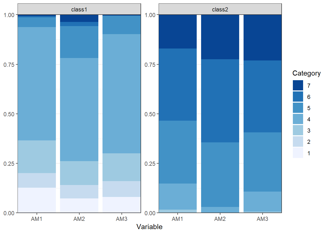
We see that the majority of people in class 1 scored a 4 on all indicators, and the majority of people in class 2 scored a 5 or 6 on all indicators. Thus, we could call these classes the “moderate AM” class, and the “high AM” class, respectively.
We can also plot this information, leading to the same conclusion:
1.8 Dichotomous indicators: mx_lca()
The Zhao dataset does not contain any binary indicators. To practice LCA with binary indicators, we will dichotomize the indicators from the previous example to practice.
Note that in real-world analyses, one should (almost) never artificially dichotomize variables, because this loses information. Because we saw that the main differences between the two classes in the previous example was between people scoring mostly 4 (class 1) versus 5 and 6 (class 2), it makes sense to cut the variables at this value:
1.8.1 Model Fitting
The number of parameters is calculated the same as for the other ordinal LCA example, but now, the number of levels L is 2. If we divide the number of cases by the number of parameters, we see that we could estimate up to 4 classes while still having, on average, about 20 observations per parameter:
 [1] 96.666667 41.428571 26.363636 19.333333 15.263158 12.608696 10.740741
 [8]  9.354839  8.285714  7.435897
We can fit the model:
| Name | Classes | LL | n | Parameters | AIC | BIC | saBIC | Entropy | prob_min | prob_max | n_min | n_max | np_ratio | np_local |
|---|---|---|---|---|---|---|---|---|---|---|---|---|---|---|
| 1 | 1 | -597.1057 | 290 | 3 | 1200.2115 | 1211.2211 | 1201.7076 | 1.0000000 | 1.0000000 | 1.0000000 | 1.0000000 | 1.0000000 | 96.66667 | 96.66667 |
| 2 | 2 | -459.3672 | 290 | 7 | 932.7345 | 958.4236 | 936.2254 | 0.9147806 | 0.9733905 | 0.9866516 | 0.4379310 | 0.5620690 | 41.42857 | 42.33333 |
| 3 | 3 | -451.2779 | 290 | 11 | 924.5559 | 964.9246 | 930.0416 | 0.7583881 | 0.8064599 | 0.9917367 | 0.2896552 | 0.3620690 | 26.36364 | 28.00000 |
| 4 | 4 | -451.2779 | 290 | 15 | 932.5559 | 987.6041 | 940.0364 | 0.5838172 | 0.4351570 | 1.0000000 | 0.1310345 | 0.3724138 | 19.33333 | 12.66667 |
Here, we see that the 2-class solution is best according to the BIC, and that np_local is near-zero for the 3- and 4-class solution. This is happens because (almost) no observations are allocated to those classes, see n_min. Thus, these classes are superfluous.
We can examine the results for the 2-class solution. Note that, because there are only two response categories, we can ignore half the table because the response proportions sum to 1, so half the rows are just one minus the other half of the rows. The table now only shows what percentage of participants scored 1 on each indicator:
| Variable | Probability | group | |
|---|---|---|---|
| 2 | AM1 | 0.86 | class1 |
| 4 | AM2 | 0.72 | class1 |
| 6 | AM3 | 0.90 | class1 |
| 8 | AM1 | 0.15 | class2 |
| 10 | AM2 | 0.01 | class2 |
| 12 | AM3 | 0.00 | class2 |
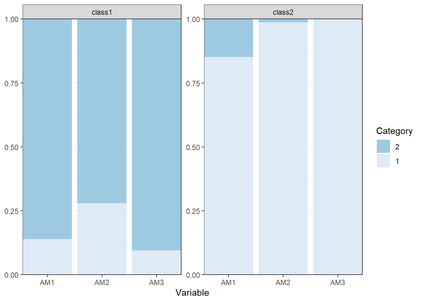
We see that people in class 2 tend to score 1 more often than people in class 1. This tells us that AM1 is most discriminating (nearly all people in class 2 endorse it, but nearly nobody in class 1), whereas AM2 is less discriminating.
We can also plot this information:
1.9 Mixed indicator types: mx_mixed_lca()
Many applied datasets contain continuous outcomes alongside ordered or binary indicators. mx_mixed_lca() is designed for this setting. As an example, we can combine df_bin with the scale score of CM:
The parameters are now given as:
- k-1 mixture weights
- k((L-1)ncol(df_lca)) thresholds
- k means for CM
- 1 variance for CM (if we keep it constant across classes)
- No covariances
 [1] 58.000000 29.000000 19.333333 14.500000 11.600000  9.666667  8.285714
 [8]  7.250000  6.444444  5.800000
So following our rule of thumb, we could safely estimate up to 3 classes:
| Name | Classes | LL | n | Parameters | AIC | BIC | saBIC | Entropy | prob_min | prob_max | n_min | n_max | np_ratio | np_local |
|---|---|---|---|---|---|---|---|---|---|---|---|---|---|---|
| equal | 1 | -1036.9096 | 290 | 5 | 2083.819 | 2102.169 | 2086.313 | 1.0000000 | 1.0000000 | 1.0000000 | 1.0000000 | 1.0000000 | 58.00000 | 58.000000 |
| equal1 | 2 | -872.4004 | 290 | 10 | 1764.801 | 1801.500 | 1769.788 | 0.8734285 | 0.9693051 | 0.9752108 | 0.4965517 | 0.5034483 | 29.00000 | 32.000000 |
| equal2 | 3 | -869.7815 | 290 | 15 | 1769.563 | 1824.611 | 1777.043 | 0.9273675 | 0.8649222 | 0.9984559 | 0.1068966 | 0.4862069 | 19.33333 | 7.153846 |
Here, we see that the 2-class solution is best according to the BIC, and that np_local is low for the 3-class solution. We can examine the results for the 2-class solution. Note that these results will now be a combination of means/variances and probabilities (thresholds):
| label | est_sig | se | pval | confint | class |
|---|---|---|---|---|---|
| Means.CM.class1 | 3.52*** | 0.09 | 0.00 | [3.35, 3.70] | class1 |
| Variances.CM.class1 | 1.05*** | 0.09 | 0.00 | [0.88, 1.23] | class1 |
| Variances.AM1.class1 | 1.00 | NA | NA | NA | class1 |
| Variances.AM2.class1 | 1.00 | NA | NA | NA | class1 |
| Variances.AM3.class1 | 1.00 | NA | NA | NA | class1 |
| class1.Thresholds[1,1].class1 | -1.60*** | 0.20 | 0.00 | [-2.00, -1.21] | class1 |
| class1.Thresholds[1,2].class1 | -0.82*** | 0.13 | 0.00 | [-1.08, -0.56] | class1 |
| class1.Thresholds[1,3].class1 | -1.38*** | 0.19 | 0.00 | [-1.75, -1.02] | class1 |
| Means.CM.class2 | 2.71*** | 0.09 | 0.00 | [2.54, 2.89] | class2 |
| Variances.AM1.class2 | 1.00 | NA | NA | NA | class2 |
| Variances.AM2.class2 | 1.00 | NA | NA | NA | class2 |
| Variances.AM3.class2 | 1.00 | NA | NA | NA | class2 |
| class2.Thresholds[1,1].class2 | 1.02*** | 0.15 | 0.00 | [0.72, 1.32] | class2 |
| class2.Thresholds[1,2].class2 | 1.86*** | 0.27 | 0.00 | [1.33, 2.39] | class2 |
| class2.Thresholds[1,3].class2 | 1.24*** | 0.16 | 0.00 | [0.92, 1.56] | class2 |
| equal var 2.weights[1,1].NA | 1.00 | NA | NA | NA | NA |
| equal var 2.weights[1,2].NA | 0.97*** | 0.13 | 0.00 | [0.72, 1.22] | NA |
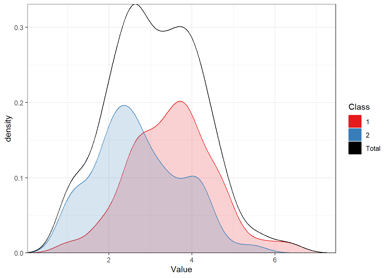
We can plot the continuous indicators:
And the response probabilities for the binary indicators:
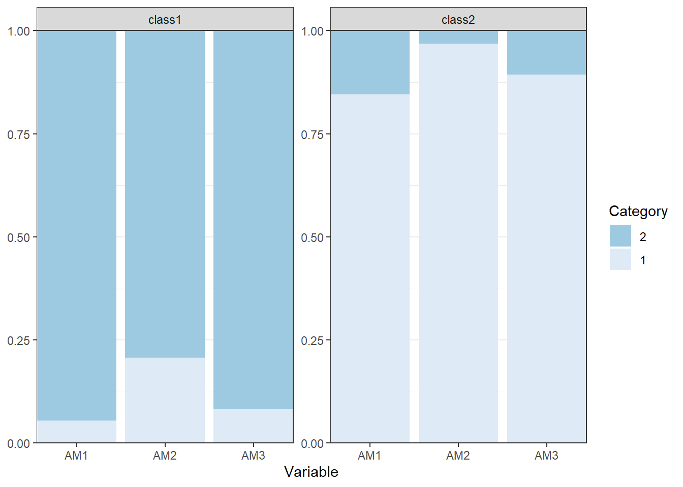
The interpretation now depends on the indicator: describe class-specific means for continuous variables, response-category probabilities for ordinal variables, and endorsement probabilities for dichotomous variables.
1.10 Classification Accuracy Deep Dive
After estimating a mixture model, every participant has a vector of posterior class-membership probabilities (i.e., the probability that they belong to each class). The function class_prob() gives you this matrix, and several other diagnostic tables based on it:
     class1 class2 class3 predicted
[1,] "0.00" "1.00" "0.00" "2.00"
[2,] "0.00" "0.00" "1.00" "3.00"
[3,] "0.99" "0.01" "0.00" "1.00"
[4,] "0.00" "1.00" "0.00" "2.00"
[5,] "0.76" "0.00" "0.24" "1.00"
[6,] "0.71" "0.29" "0.00" "1.00"
This table can be summarized in different ways to summarize the classifications, and to diagnose classification accuracy.
For example, $sum.posterior gives us the column sums of the individual classification probabilities; this indicates what proportion of your sample contributes to each class (and allows people to contribute fractionally to multiple classes):
| class | count | proportion |
|---|---|---|
| class1 | 171.83 | 0.59 |
| class2 | 88.42 | 0.30 |
| class3 | 29.75 | 0.10 |
If you make a forced choice, assigning every person to the class for which they have the highest probability, you would get the following statistics. Note that these numbers now have measurement error baked into them:
| class | count | proportion |
|---|---|---|
| class1 | 178 | 0.61 |
| class2 | 84 | 0.29 |
| class3 | 28 | 0.10 |
In Section 1.6.4, we already encountered the average classification probabilities for the most likely class membership, whose range is represented in the fit table as prob_min and prob_max. We can see the full matrix by calling:
          assigned.1 assigned.2 assigned.3
avgprob.1 "0.95"     "0.04"     "0.01"
avgprob.2 "0.13"     "0.87"     "0.00"
avgprob.3 "0.12"     "0.00"     "0.88"
On the diagonal, we find the average probability that observations belongs to the classes they are assigned to. If the classes are well-separated, you should see large diagonal values and small off-diagonal values. The separation here is OK; some diagonal values are not that high (.87-.88), and some off-diagonal values are non-negligible (.12-.13). For instance, you see that the people who are assigned to class 1 have an average posterior probability of .95 for belonging to that class - which is very high. However, they also have non-zero probabilities of belonging to class 2 or 3.
Quiz
Person A has classification probabilities (.41, .34, .25). This person belongs to class:
Person B has classification probabilities (.92, .06, .02). Which person can be classified with greater certainty?
If you treat class membership as observed in follow-up analyses, your standard errors will be too small.
You can generally use most likely class membership as a predictor or covariate to perform follow-up analyses to compare classes, e.g., with ANOVA or regression.
If prob_min and prob_max are .99 and 1.00, it's fine to treat most likely class membership as an observed variable in follow-up analyses.
1.11 Reporting Results
Going back to the LPA example from Section 1.6, you might report the analysis as follows:
We conducted exploratory latent profile analysis using
tidySEMversion 0.2.12 andOpenMxversion 2.22.11. We followed recommended practices by Van Lissa et al. (2024). The two continuous indicators were AM and CM. Model parameters were class-varying means and fixed variances across classes. We assumed conditional independence of these indicators within classes. Based on the available sample size, we considered a maximum of five classes. This model has 16 parameters, which allows for a maximum of about 20 observations per parameter. We selected the best-fitting model based on the BIC and significant BLRT test. We eliminated solutions with classes where the number of observations to parameters was smaller than 10. Based on these criteria, a 3-class solution was retained. This model had reasonable classification accuracy: entropy was .82, and the probability that observations in each class were correctly classified ranged from [.87, .95]. The smallest class contained 9.7% of participants. The model parameters are show in Table 1, and are visually represented in Figure 1. The retained classes were characterized as [label 1], [label 2], and [label 3] based on their estimated [means / category-response probabilities / endorsement probabilities].
Here is the code to produce Table 1; we extract the means and paste the SE behind it (note that you can also use est_sig or another value column). We do not report the variances in this table, because they are fixed across classes. We also write it to a spreadsheet, so we can easily import it into other desktop publishing software:
tab <- table_results(res_lpa[[2]], columns = NULL)
tab <- tab[tab$Category == "Means", c("lhs", "class", "est", "se")]
tab$Mean <- glue::glue("{tab$est} ({tab$se})")
tab <- reshape(tab[, c("class", "lhs", "Mean")], direction = "wide", idvar = "class", timevar = "lhs", sep = " ")
write.csv(tab, "tab_res.csv", row.names = FALSE)
tab| class | Mean AM | Mean CM | |
|---|---|---|---|
| 1 | class1 | 2.83 (0.42) | 4.14 (0.19) |
| 5 | class2 | 5.01 (0.11) | 2.90 (0.10) |
To produce Figure 1, use the following code. We’re saving the file to SVG format, which is a (lossless) type of vector graphic. Other vector graphic types include PDF and EPS. Do not save to a raster graphic type (PNG, BMP, JPG), because these images will have low quality when reproduced in print or digital publication. The dimensions of the figure, in millimeter, correspond to A6 paper format: