2 Confirmatory Latent Class Analysis

Latent profile analysis (LPA) is often used exploratorily: researchers estimate several class solutions and then decide which one best describes the data. But LPA can also be used confirmatorily, when theory makes specific predictions about the latent class structure.

To follow along and run the code yourself, open the file lca_confirmatory.qmd in the lca_course project, as explained in Appendix A.

In this first example, suppose that clinical psychological theory proposes the existence of two subpopulations:

people without depression
people with depression

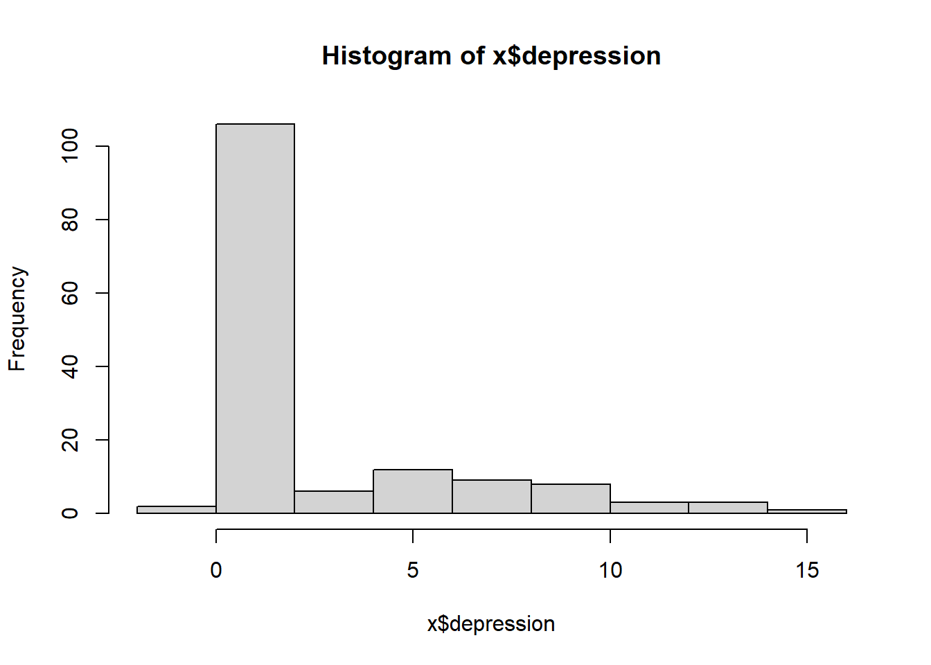
If all we know is people’s depression score, then we can try to identify two latent classes, corresponding to these subpopulations. Suppose that the theory further specifies that a depression score of about 10 or higher is required to count as depressed. We will use this theory to formulate two increasingly specific hypotheses:

a two-class model should fit better than a one-class model. Adding a third class should not significantly improve fit.
the class means should be close to 0 for the non-depressed class and 10 for the depressed class.

The second hypothesis is considerably stronger because it constrains the class-specific means to exact values.

2.1 Simulate example data

We first create a simple dataset containing a single continuous depression score.

library(tidySEM)
library(OpenMx)

set.seed(123)
x <- data.frame(
  depression = c(
     # The people with depression:
    rnorm(50, mean = 6, sd = 4),
    # The people without depression:
    rbeta(100, 2, 3)
  )
)
hist(x$depression)

2.2 Test the number of classes

The first confirmatory hypothesis concerns class enumeration. Theory predicts two classes, so we estimate one-, two-, and three-class solutions.

res <- mx_profiles(
  x,
  classes = 1:3
)
saveRDS(res, "res_depression.rds")

res <- readRDS("res_depression.rds")
table_fit(res)

Name	Classes	LL	n	Parameters	AIC	BIC	saBIC	Entropy	prob_min	prob_max	n_min	n_max	np_ratio	np_local
equal var 1	1	-398.3120	150	2	800.6240	806.6453	800.3156	1.0000000	1.0000000	1.0000000	1.0000000	1.0000000	75.0	75.00000
equal var 2	2	-346.5824	150	4	701.1647	713.2072	700.5480	0.9495445	0.9432520	0.9953478	0.1733333	0.8266667	37.5	17.33333
equal var 3	3	-314.9716	150	6	641.9432	660.0070	641.0182	0.9658533	0.9590919	0.9889837	0.1200000	0.7200000	25.0	13.50000

The fit table lets us inspect information criteria and other model-fit statistics across the competing class solutions.

If we want to test the theory, we can compare adjacent class solutions using the bootstrapped likelihood ratio test (BLRT).

res_blrt <- BLRT(res)
saveRDS(res_blrt, "blrt_depression.rds")

res_blrt <- readRDS("blrt_depression.rds")
res_blrt

	null	alt	lr	df	blrt_p	samples
equal var 1	mix1	mix2	103.45929	2	0	67
equal var 2	mix2	mix3	63.22149	2	0	91

Quiz

According to BIC, the best-fitting model is:
According to BLRT, the two-class model fits significantly better than the 1- and 3-class model.

2.3 Translate theoretical assumptions into parameter constraints

The models above still allow all parameters to be estimated freely from the data. That tests only the broad hypothesis that two groups exist. The groups themselves could diverge substantially from what was theorized.

Our theory posits that the non-depressed class should have a mean near 0, whereas the depressed class should have a mean near 10 (technically, the minimum value in that class should be 10, but that’s a bit more difficult to enforce).

We can represent this stronger hypothesis by fixing the two class means to these values, or by e.g. setting a parameter constraint for the two classes.

First, create the two-class profile model without estimating it and examine its parameters:

res_theory <- mx_profiles(
  x,
  classes = 2,
  run = FALSE
)
omxGetParameters(res_theory)

equal var 2.weights[1,2]                       v1                      m11 
               0.2605042                2.3038225                0.7251967 
                     m21 
               8.3585995

The relevant mean parameters are m11 and m21. We can either fix these means to the exact values of 0 and 10:

res_theory <- omxSetParameters(
  res_theory,
  labels = c("m11", "m21"),
  values = c(0, 10),
  free = FALSE
)

Or alternatively, we could set a lower and upper bound for these parameters, thus allowing bounded free estimation:

res_theory_bounds <- omxSetParameters(
  res_theory,
  labels = c("m11", "m21"),
  values = c(0, 10),
  free = TRUE,
  lbound = c(NA, 10),
  ubound = c(1, NA)
)

Now, run your chosen model:

res_theory <- run_mx(res_theory)
res_theory_bounds <- run_mx(res_theory_bounds)

Next, compare the unconstrained two-class solution with the theory-constrained model.

compare_these <- list(
  res[[2]],
  res_theory,
  res_theory_bounds
)

table_fit(compare_these)

Name	Classes	LL	n	Parameters	AIC	BIC	saBIC	Entropy	prob_min	prob_max	n_min	n_max	np_ratio	np_local
1	2	-346.5824	150	4	701.1647	713.2072	700.5480	0.9495445	0.9432520	0.9953478	0.1733333	0.8266667	37.5	17.33333
2	2	-368.6431	150	2	741.2862	747.3075	740.9778	0.9488272	0.9595115	0.9918444	0.1733333	0.8266667	75.0	52.00000
3	2	-350.6497	150	4	709.2994	721.3419	708.6827	0.9599385	0.9670867	0.9939682	0.1600000	0.8400000	37.5	16.00000

We can also compare the models using the BLRT:

blrt_theory <- BLRT(list(res[[2]], res_theory))
saveRDS(blrt_theory, "blrt_theory.rds")

blrt_theory <- readRDS("blrt_theory.rds")
blrt_theory

	null	alt	lr	df	blrt_p	samples
2	mix2	equal var 2	-44.12149	-2	0.47	100

Note that fixing the class means to exact values is a very strong assumption. In many real applications, theory may imply that class means should be near certain values rather than exactly equal to them. You can also manually specify start values, and then test if the estimated parameter values deviate significantly from these:

res_theory_starts <- omxSetParameters(
  res_theory,
  labels = c("m11", "m21"),
  values = c(0, 10),
  free = TRUE
)
res_theory_starts <- run_mx(res_theory_starts)
omxGetParameters(res_theory_starts)

equal var 2.weights[1,2]                       v1                      m11 
               0.2190895                2.4874123                0.8699903 
                     m21 
               8.8424735

wald_test(res_theory_starts, "m11 = 0; m21 = 10")

NULL

Quiz

According to the BIC, which model is best?
According to the BLRT, we should prefer the constrained model to the free model.
According to the Wald test, the mean of class 2 is not significantly different from 10.

3 Caregiver Compass

For this next example, we will use simulated data based on work by Zegwaard and colleagues, who sought to establish a typology of caregivers who support a close other receiving outpatient psychological care. Qualitative research among experts resulted in a theory postulating the existence of four types of caregivers (translated from the original Dutch):

Balanced

The balanced caregiver experiences relative balance between the costs and benefits of caring for a close other.

Imbalanced

The imbalanced caregiver experiences a precarious balance between the costs and benefits of caring for a close other.

Lonely

The lonely caregiver experiences a strong sense of isolation.

Entrapped

The entrapped caregiver strongly feels a sense of being entangled in responsibilities which are difficult to fulfill.

The goal of this confirmatory study was to validate this hypothesized class solution in a sample of caregivers. A convenience sample was used, with no prior sample size justification. To view the data documentation, run the command ?tidySEM::zegwaard_carecompass in the R console.

3.1 Loading the Data

To load the data, simply attach the tidySEM package. For convenience, we assign the variables used for analysis to an object called df. We first only use the four scales: c("burdened", "trapped", "negaffect", "loneliness").

# Load required packages
library(tidySEM) 
library(ggplot2)
library(OpenMx)
library(scales)
library(mice)
# Load data
df <- zegwaard_carecompass[, c("burdened", "trapped", "negaffect", "loneliness")]

3.2 Descriptive statistics

We use tidySEM::descriptives() to describe the data numerically. Because all scales are continuous, we select only columns for continuous data to de-clutter the table:

desc <- tidySEM::descriptives(df)
desc <- desc[, c("name", "n", "missing", "unique",
                 "mean", "median", "sd", "min", "max",
                 "skew_2se", "kurt_2se")]
desc

name	n	missing	unique	mean	median	sd	min	max	skew_2se	kurt_2se
burdened	509	0.0077973	509	3.383978	3.385765	0.7468695	1.1958284	5.282460	0.1723420	-0.4102692
trapped	505	0.0155945	505	1.725223	1.787354	0.8976391	-0.8578806	3.805728	-1.0343850	-1.5170521
negaffect	506	0.0136452	506	2.502401	2.519129	0.6901424	0.7086115	4.983359	0.0843737	-0.3823452
loneliness	510	0.0058480	510	2.658997	2.692829	0.6176745	0.9845240	4.217298	-0.3266117	-0.6222047

The table indicates two potential causes for concern: there is a small percentage of missingness, and all variables have relatively high kurtosis. Since there are some missing values, we can conduct an MCAR test using mice::mcar(df):

test_mcar <- mcar(df)


 iter imp variable
  1   1  burdened  trapped  negaffect  loneliness
  1   2  burdened  trapped  negaffect  loneliness
  1   3  burdened  trapped  negaffect  loneliness
  1   4  burdened  trapped  negaffect  loneliness
  1   5  burdened  trapped  negaffect  loneliness
  2   1  burdened  trapped  negaffect  loneliness
  2   2  burdened  trapped  negaffect  loneliness
  2   3  burdened  trapped  negaffect  loneliness
  2   4  burdened  trapped  negaffect  loneliness
  2   5  burdened  trapped  negaffect  loneliness
  3   1  burdened  trapped  negaffect  loneliness
  3   2  burdened  trapped  negaffect  loneliness
  3   3  burdened  trapped  negaffect  loneliness
  3   4  burdened  trapped  negaffect  loneliness
  3   5  burdened  trapped  negaffect  loneliness
  4   1  burdened  trapped  negaffect  loneliness
  4   2  burdened  trapped  negaffect  loneliness
  4   3  burdened  trapped  negaffect  loneliness
  4   4  burdened  trapped  negaffect  loneliness
  4   5  burdened  trapped  negaffect  loneliness
  5   1  burdened  trapped  negaffect  loneliness
  5   2  burdened  trapped  negaffect  loneliness
  5   3  burdened  trapped  negaffect  loneliness
  5   4  burdened  trapped  negaffect  loneliness
  5   5  burdened  trapped  negaffect  loneliness

test_mcar


Missing data patterns: 3 used, 3 removed.
Cases used: 506 

Hawkins' test: median chi^2 (6) = 4.369945, median p = 0.626746


Interpretation of results:
 Hawkins' test is not significant; there is no evidence to reject the assumptions of multivariate normality and MCAR.

You should find that, according to Hawkins’ test, there is no evidence to reject the assumptions of multivariate normality and MCAR. In tidySEM, missing data is accounted for using FIML by default, meaning that available data will be used without imputation. This is appropriate if data are missing completely at random, or if the missingness is contingent on the observed variables - but not if missingness is contingent on the missing data (which is impossible to diagnose, and for which no adequate solution exists).

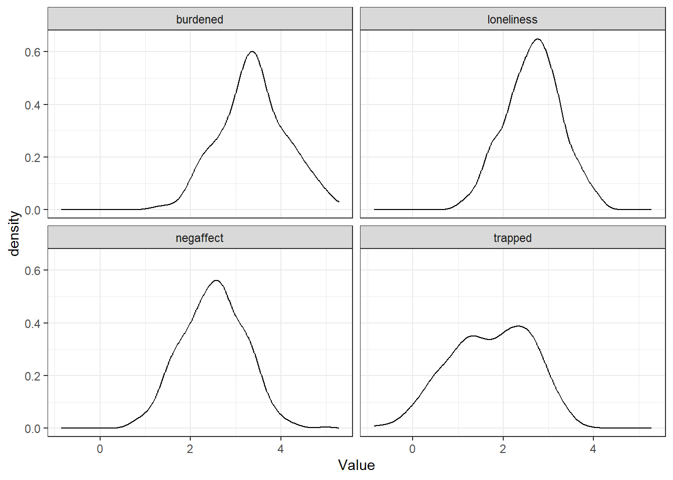
Additionally, we can plot the data. The ggplot2 function geom_density() is useful for continuous data. Visual inspection confirms the conclusions from the descriptives() table: the data are kurtotic (peaked).

df_plot <- df
names(df_plot) <- paste0("Value.", names(df_plot))
df_plot <- reshape(df_plot, varying = names(df_plot), direction = "long",
                   timevar = "Variable")
ggplot(df_plot, aes(x = Value)) +
  geom_density() +
  facet_wrap(~Variable)+
  theme_bw()

3.3 Conducting Latent Profile Analysis

As all variables are continuous, we can use the convenience function tidySEM::mx_profiles(), which is a wrapper for the generic function mx_mixture() optimized for continuous indicators. Its default settings are appropriate for LPA, assuming fixed variances across classes and zero covariances. Its arguments are data and number of classes. All variables in data are included in the analysis, which is why we first selected the indicator variables. As this is a confirmatory LCA, we do not follow a strictly data-driven class enumeration procedure. We will set the maximum number of classes \(K\) to one more than the theoretically expected number. We set a seed to ensure replicable results.

set.seed(123) # setting seed 
res <- mx_profiles(data = df,
                   classes = 1:5)
saveRDS(res, "res_conf.rds")

res <- readRDS("res_conf.rds")

This analysis should produce some messages about cluster initialization. These relate to the selection of starting values, which relies on the K-means algorithm and is not robust to missing data. The algorithm automatically switches to hierarchical clustering, no further action is required.

3.4 Class Enumeration

To compare the fit of the theoretical model against other models, we create a model fit table using table_fit() and retain relevant columns. We also determine whether any models can be disqualified.

In this example, all models converge without issues. If, for example, the two-class solution had not converged, we could use the function res[[2]] <- mxTryHard(res[[2]]) to aid convergence.

Next, we check for local identifiability. The sample size is consistently reported as 513, which means that partially missing cases were indeed included via FIML. The smallest class size occurs in the 5-class model, where the smallest class is assigned 7% of cases, or 38 cases. This model has 28 parameters, approximately 6 per class. We thus have at least five observations per parameter in every class, and do not disqualify the 5-class model.

There are concerns about theoretical interpretability of all solutions, as the entropies and minimum classification probabilities are all low. However, in this confirmatory use case, we address this when interpreting the results.

fit <- table_fit(res) # model fit table
fit[ , c("Name", "LL", "Parameters", "n",
         "BIC", "Entropy",
         "prob_min", "prob_max", 
         "n_min", "n_max",
         "np_ratio", "np_local")]

Name	LL	Parameters	n	BIC	Entropy	prob_min	prob_max	n_min	n_max	np_ratio	np_local
equal var 1	-2241.982	8	513	4533.886	1.0000000	1.0000000	1.0000000	1.0000000	1.0000000	64.12500	64.1250000
equal var 2	-2031.365	13	513	4143.854	0.7404912	0.9116044	0.9298845	0.4191033	0.5808967	39.46154	35.8333333
equal var 3	-1951.349	18	513	4015.023	0.7797238	0.8860997	0.9146913	0.1871345	0.5438596	28.50000	18.0000000
equal var 4	-1916.253	23	513	3976.033	0.7548658	0.8142116	0.9151926	0.1559454	0.3430799	22.30435	16.0000000
equal var 5	-1912.370	28	513	3999.469	0.7878139	0.8109998	0.9155951	0.0038986	0.3411306	18.32143	0.4166667

3.4.1 Using ICs

the 4-class solution has the lowest BIC, which means it is preferred over all other solutions including a 1-class solution and a solution with more classes. Note that a scree plot for the BIC can be plotted by calling plot(fit). Following the elbow criterion, a three-class solution would also be defensible. The function ic_weights(fit) allows us to compute IC weights; it indicates that, conditional on the set of models, the 4-class model has a posterior model probability of nearly 100%.

3.4.2 Using LMR tests

Note that the use of LMR tests is discouraged; these tests make assumptions that are known to be violated for latent class analyses (Van Lissa et al., 2024). Nevertheless - if we do conduct LMR tests, we find that the tests are significant for all pairwise model comparisons, except for the 5-class model. Note that, as this analysis takes a long time, you don’t have to run it - you can load its results from a file.

test_lmr <- lr_lmr(res)
saveRDS(test_lmr, "test_lmr.rds")

test_lmr <- readRDS("test_lmr.rds")
format_numeric(test_lmr)

null	alt	lr	df	p	w2
mix1	mix2	10.25	5	0.00	0.82
mix2	mix3	5.30	5	0.00	0.44
mix3	mix4	4.14	5	0.00	0.14
mix4	mix5	0.88	5	0.19	0.04

3.4.3 Using BLRT tests

We can also use the BLRT test, which is the best practice solution for class enumeration, but is very computationally expensive. You can load the test results from a file, and we used a low number of replications to make it more feasible. In practice, one might use a much higher number (1000+) for published research. Keep in mind that the p-value of the BLRT is subject to Monte Carlo error; if it fluctuates when analyses are replicated or its value is very close to the critical threshold, consider increasing the number of replications.

To accelerate computations, we can use the future package for parallel computing (see ?plan to select the appropriate back-end for your system). To track the function’s progress, we use the progressr ecosystem, which allows users to choose how they want to be informed. The example below uses a progress bar:

library(future)
library(progressr)
plan(multisession) # Parallel processing for Windows
handlers("progress") # Progress bar
set.seed(1)
test_blrt <- BLRT(res, replications = 100)
saveRDS(test_blrt, "test_blrt.rds")

test_blrt <- readRDS("test_blrt.rds")
format_numeric(test_blrt)

	null	alt	lr	df	blrt_p	samples
equal var 1	mix1	mix2	421.23	5	0.00	100
equal var 2	mix2	mix3	160.03	5	0.00	100
equal var 3	mix3	mix4	70.19	5	0.00	100
equal var 4	mix4	mix5	7.77	5	0.36	100

In sum, across all class enumeration criteria, there is strong support for a 4-class solution.

3.5 Comparing Competing Theoretical Model Specifications

In the case of confirmatory LCA, the theory would be refuted by strong evidence against the hypothesized model and number of classes. In the preceding, we only compared the theoretical model against models with different number of classes. Imagine, however, that a Reviewer argues that variance ought to be freely estimated across classes. We could compare our theoretical model against their competing model as follows. Note that we can put two models into a list to compare them.

res_alt <- mx_profiles(df, classes = 4, variances = "varying")
saveRDS(res_alt, "res_alt.rds")

res_alt <- readRDS("res_alt.rds")
compare <- list(res[[4]], res_alt)
table_fit(compare)

Name	Classes	LL	n	Parameters	AIC	BIC	saBIC	Entropy	prob_min	prob_max	n_min	n_max	np_ratio	np_local
1	4	-1916.253	513	23	3878.507	3976.033	3903.028	0.7548658	0.8142116	0.9151926	0.1559454	0.3430799	22.30435	16.00
2	4	-1909.232	513	35	3888.464	4036.874	3925.778	0.7816344	0.8445960	0.9210385	0.1598441	0.3157895	14.65714	10.25

The alternative model incurs 12 additional parameters for the free variances. Yet, it has a higher BIC, which indicates that this additional complexity does not outweigh the increase in fit.

You can obtain a significance test for this model comparison by using the BLRT:

test_compare <- BLRT(compare, replications = 100)
saveRDS(test_compare, "test_compare.rds")

test_compare <- readRDS("test_compare.rds")
test_compare

	null	alt	lr	df	blrt_p	samples
2	mix4	free var 4	14.04277	12	0.39	100

3.6 Interpreting the Final Class Solution

To interpret the final class solution, we first reorder the 4-class model by class size. This helps prevent label switching.

res_final <- mx_switch_labels(res[[4]])

The 4-class model yielded classes of reasonable size; the largest class comprised 33%, and the smallest comprised 16% of cases. However, the entropy was low, \(S = .75\), indicating poor class separability. Furthermore, the posterior classification probability ranged from \([.81, .92]\), which means that at least some classes had a high classification error. We produce a table of the results below.

table_results(res_final, columns = c("label", "est", "se", "confint", "class"))

label	est	se	confint	class
Means.burdened.class1	3.27	0.04	[3.18, 3.36]	class1
Means.trapped.class1	1.28	0.05	[1.18, 1.38]	class1
Means.negaffect.class1	2.31	0.06	[2.20, 2.42]	class1
Means.loneliness.class1	2.73	0.04	[2.64, 2.82]	class1
Variances.burdened.class1	0.23	0.02	[0.19, 0.27]	class1
Variances.trapped.class1	0.17	0.02	[0.14, 0.20]	class1
Variances.negaffect.class1	0.31	0.02	[0.27, 0.36]	class1
Variances.loneliness.class1	0.24	0.02	[0.20, 0.28]	class1
Means.burdened.class2	3.40	0.06	[3.28, 3.52]	class2
Means.trapped.class2	2.27	0.06	[2.15, 2.38]	class2
Means.negaffect.class2	2.81	0.06	[2.70, 2.93]	class2
Means.loneliness.class2	2.79	0.06	[2.66, 2.91]	class2
Means.burdened.class3	4.25	0.07	[4.12, 4.38]	class3
Means.trapped.class3	2.67	0.05	[2.58, 2.77]	class3
Means.negaffect.class3	2.92	0.06	[2.80, 3.03]	class3
Means.loneliness.class3	2.01	0.06	[1.89, 2.14]	class3
Means.burdened.class4	2.38	0.06	[2.26, 2.50]	class4
Means.trapped.class4	0.38	0.05	[0.28, 0.49]	class4
Means.negaffect.class4	1.78	0.07	[1.65, 1.91]	class4
Means.loneliness.class4	3.18	0.06	[3.07, 3.30]	class4
mix4.weights[1,1].NA	1.00	NA	NA	NA
mix4.weights[1,2].NA	0.86	0.15	[0.56, 1.15]	NA
mix4.weights[1,3].NA	0.66	0.11	[0.44, 0.88]	NA
mix4.weights[1,4].NA	0.47	0.08	[0.32, 0.63]	NA

The results are best interpreted by examining a plot of the model and data, however. Relevant plot functions are plot_bivariate(), plot_density(), and plot_profiles(). However, we omit the density plots, because plot_bivariate() also includes them.

plot_bivariate(res_final)

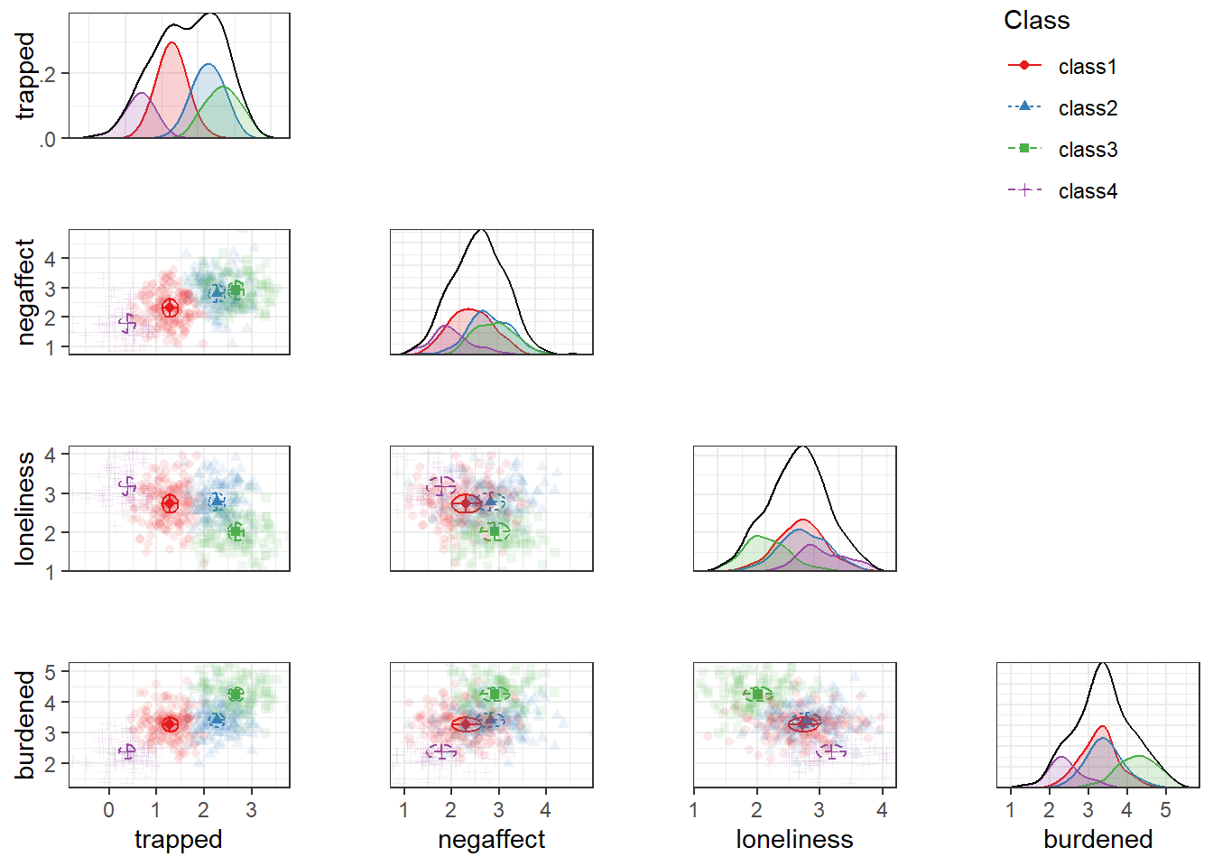
On the diagonal of the bivariate plot are weighted density plots: normal approximations of the density function of observed data, weighed by class probability. On the off-diagonal are plots for each pair of indicators, with the class means indicated by a point, class standard deviations indicated by lines, and covariances indicated by circles. As this model has zero covariances, all circles are round (albeit warped by the different scales of the X and Y axes)

The marginal density plots show that trappedness distinguishes classes rather well. For all other indicators, groups are not always clearly separated in terms of marginal density: class 2 and 3 coalesce on negative affect, 1 and 2 coalesce on loneliness, and 1 and 2 coalesce on burden. Nevertheless, the off-diagonal scatterplots show reasonable bivariate separation for all classes.

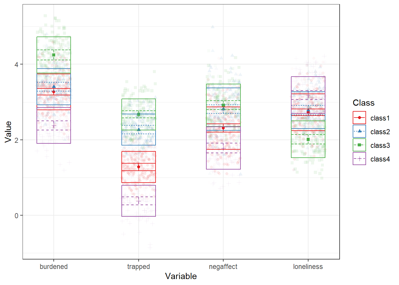
We can obtain a more classic profile plot using plot_profiles(res_final). This plot conveys less information than the bivariate plot, but is readily interpretable. Below is a comparison between the most common type of visualization for LPA, and the best-practices visualization provided by tidySEM. Note that the best practices plot includes class means and error bars, standard deviations, and a ribbon plot of raw data weighted by class probability to indicate how well the classes describe the observed distribution. The overlap between the classes is clearly visible in this figure; this is why the entropy and classification probabilities are relatively low.

Based on the bivariate plot, we can label class 1 as the balanced type (33%), class 2 as the imbalanced type (29%), class 3 as the entrapped type (22%), and class 4 as the lonely type (16%). Note however that the observed classes do not match the hypothesized pattern of class parameters exactly.

plot_profiles(res_final)

We will save the final model for future reference:

saveRDS(res_final, "res_zegwaard.rds")