In previous chapters, we have explored various regression techniques, including bivariate linear regression, independent samples t-tests, and analysis of variance (ANOVA). We’ve also delved into the concept of interaction between binary and continuous predictors. In this chapter, we build upon that prior knowledge when explaining the Factorial ANOVA.
Factorial ANOVA is used to examine the effects of multiple categorical predictors and their interactions on a continuous outcome variable. Despite its historical development as a separate method, factorial ANOVA can be conceptualized as a special case of multiple regression. It combines the concepts of dummy coding and interaction that we’ve previously encountered. Each factor is represented via dummy coding, and creating interaction terms are computed by multiplying those dummies.
The reason ANOVA is often considered a separate technique is that it has different historical roots from regression, and because of those roots, researchers typically focus on different output when reporting factorial ANOVA versus regression. For example, ANOVA focuses more on variance explained by each factor, and overall tests of the effect of each Factor across all of its levels.
A factorial ANOVA involves two or more factors, each with multiple levels. Each combination of factor levels creates a unique condition or group in the study. For instance, if we have Factor A with 3 levels and Factor B with 2 levels, the factorial design will have a total of 3 × 2 = 6 groups.
Factorial designs can be visually represented in a matrix-like structure, where each cell represents a unique combination of factor levels. This representation helps us understand the experimental conditions and the interactions between factors.
In factorial ANOVA, we examine main effects and interaction effects. As in multiple regression, main effects represent the influence of each factor on the dependent variable, controlling for all other predictors. Interaction effects capture how the effects of one factor depend on the levels of another factor.
Because each factor may be represented by multiple dummies, we can’t use individual t-tests for the dummies to determine the siginficance of the Factor they belong to. Instead, we use F-tests to test the significance of the effect of a Factor. These F-tests compare the variance explained by the factor to the unexplained variance.
In addition to significance tests, effect size measures help us understand the practical importance of the effects observed in factorial ANOVA. Eta squared and partial eta squared are common effect size measures that quantify the proportion of variance explained by each factor or interaction, relative to the total variance or unexplained variance, respectively. Eta squared is just a different name for R squared; partial eta squared is something different, and typically only reported for ANOVA.
20.1 Lecture
20.2 Formative Test
A formative test helps you assess your progress in the course, and helps you address any blind spots in your understanding of the material. If you get a question wrong, you will receive a hint on how to improve your understanding of the material.
Complete the formative test ideally after you’ve seen the lecture, but before the lecture meeting in which we can discuss any topics that need more attention
Question 1
What is the primary objective of factorial ANOVA?
Question 2
In a 2x2 factorial design, how many unique conditions or groups are there?
Question 3
What does a main effect represent in factorial ANOVA?
Question 4
What does an interaction effect capture in factorial ANOVA?
Question 5
Which effect size measure quantifies the proportion of variance explained by each factor or interaction relative to the total variance?
Question 6
What does it mean when lines representing different conditions on a means plot cross each other?
Question 7
In a 3x2 factorial design, how many dummies would be required in total to represent both factors?
Question 8
Which term describes the variance remaining unexplained by the factors and interactions in factorial ANOVA?
Question 9
What does a partial eta squared measure in factorial ANOVA?
Question 1
Factorial ANOVA allows us to explore how multiple categorical predictors and their interactions impact a continuous outcome variable.
Question 2
In a 2x2 factorial design, there are 2 levels for Factor A and 2 levels for Factor B, resulting in a total of 2 x 2 = 4 unique conditions.
Question 3
A main effect reflects the impact of a specific factor on the dependent variable while considering the influence of other factors.
Question 4
An interaction effect in factorial ANOVA describes how the effects of one factor change based on the levels of another factor.
Question 5
Eta squared is an effect size measure in factorial ANOVA that indicates the proportion of variance explained by a factor or interaction relative to the total variance.
Question 6
Crossing lines on a means plot indicate a significant interaction between the factors, suggesting that the effect of one factor depends on the levels of another factor.
Question 7
For a 3x2 factorial design, Factor A would require 2 dummies, and Factor B would require 1 dummy. Therefore, the total number of dummies needed is 2 + 1 = 3.
Question 8
Residual variance refers to the unexplained variability in the dependent variable after accounting for the effects of factors and interactions in factorial ANOVA.
Question 9
Partial eta squared quantifies the proportion of variance explained by a specific factor while controlling for the influence of other factors in the model.
20.3 Tutorial
20.3.1 Factorial ANOVA
Consider the following research situation: A psychologist wants to study if and to what extent different behavior of waiters affect the amount of tip money they get, and whether it matters if the behavior is shown by a waiter or waitress.
The researcher distinguishes the following types of behavior: neutral behavior, drawing a smiley on the bill, or making small talk.
They ran a fully crossed experiment with 3 (behaviors) x 2 (gender: waiter or waitress) = 6 conditions. For each condition they collected data for 10 customers who were helped by a waiter showing neutral behavior, 10 helped by a waiter drawing a smiley on the bill, and so forth.
Is the design balanced?
What is/are the independent variable(s) in this experiment?
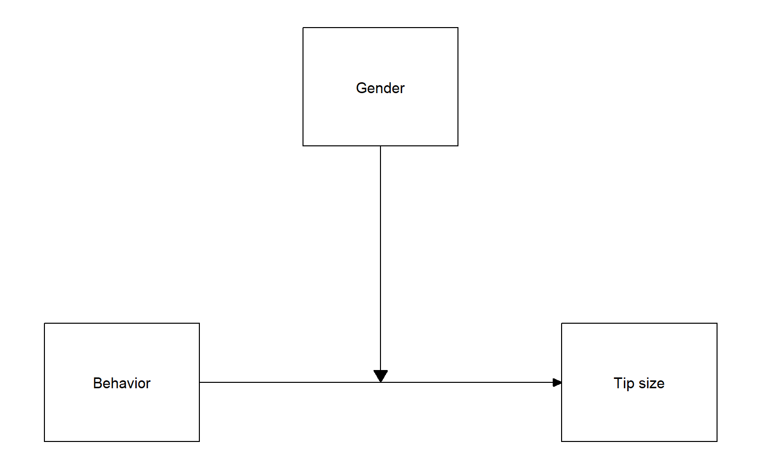
Draw the conceptual model of the experiment. Then, check your answer.
As you can see, the dependent variable is Tip money, and the independent variables are Type of behavior and Gender. More specifically. Gender is the moderator, as is expected to influence the relationship between Behavior and Tip money.
As you can see, the dependent variable is Tip money, and the independent variables are Type of behavior and Gender. More specifically. Gender is the moderator, as is expected to influence the relationship between Behavior and Tip money.
20.3.2 Regression with dummies
First, we analyze these data using regression with dummies.
You will need to dummy code both categorical predictors.
Do this in the familiar way, then check your syntax.
RECODE behavior (1=1) (2=0) (3=0) INTO talking.
RECODE behavior (1=0) (2=1) (3=0) INTO smiling.
RECODE behavior (1=0) (2=0) (3=1) INTO neutral.

RECODE Gender (1=1) (2=0) INTO waitress.
RECODE Gender (1=0) (2=1) INTO waiter.
EXECUTE.
Estimate a regression model with a main effect for gender and behavior. Create the syntax, then check your answer below.
Using neutral behavior and waiter as reference categories, the code is:
REGRESSION
  /MISSING LISTWISE
  /STATISTICS COEFF OUTS R ANOVA
  /CRITERIA=PIN(.05) POUT(.10)
  /NOORIGIN
  /DEPENDENT Tip
  /METHOD=ENTER waitress smiling talking.
Now, we want to examine whether there is an interaction between gender and behavior. To do so, we want to specify a “full factorial” model. This simply means that we want to know if there is an interaction effect between the two categorical variables. The way to include an interaction effect is to multiply the predictor. As each predictor is represented by multiple dummies, we have to multiply each dummy for each variable with all dummies from the other variable.
In this case, that means multiplying the waiter dummy with the smiling and talking dummies.
Conduct a hierarchical regression analysis that includes these new interaction terms.
What proportion of the total variance in Tip money is explained by the full factorial model?
True or false: The full factorial model explains a significant amount of variance.
Is there a significant interaction effect?
Even though we see significant interaction terms in the coefficients table, determining whether there is a significant interaction between categorical variables requires more than just “eyeballing” whether those terms are significant or not. You need to perform a nested model test.
Based on the output, complete the following table:
Behavior
Gender
Mean
Neutral
Waiter
4.600
Neutral
Waitress
Smiley
Waiter
5.100
Smiley
Waitress
7.600
Small talk
Waiter
Small talk
Waitress
10.000
Draw a rough plot of these means on a piece of paper.
Put the type of behavior on the x-axis and draw separate lines for waiters and waitresses.
True or false: The graph suggests a potential interaction.
If so, describe the interaction effect (i.e., what can we say about the effect of behavior on amount of tip money for waiters and waitresses?).
The lines are not parallel. Hence, also from the graph we see that there is interaction. The effect of type of behavior on the amount of tip money depends on the gender of the waiter/waitress.
It seems that for waiters the tip money does not depend much on the behavior.
For waitresses the effect is stronger; neutral behavior produces the least amount of tip money, whereas small talk is most beneficial.
See if you can answer the following question by yourself:
True or false: The interaction effect is significant.
To answer this question, you need to perform a nested model test.
Note two things: we request CHANGE statistics, and we enter all “interaction effects” in a separate step, so we can use the R-squared change test to determine overall significance.
What is the value of the test statistic for the significance of the interaction effect?
Report the effect, then check your answer.
There was a significant interaction effect between waiters’ sex and behavior, F(2,54) = 18.315, p < .001.
This means that the effect of Type of behavior on Tip money depends on the Gender of the waiter/waitress.
Out of curiosity - how much variance is explained by the main effects only?
20.3.3 ANOVA interface
SPSS also has a dedicated “ANOVA interface”. It specifies exactly the same model as we have been investigating, but its output is more focused on information that is typically requested when estimating a model with only categorical predictors and (optionally) interactions between them.
We will now use the ANOVA interface and pay special attention to output it gives us that is not directly available via the Regression interface.
You can either use the graphical user interface, or copy-paste this syntax. Either way, pay particular attention to the following:
Under Options, ask for Homogeneity tests: /PRINT=HOMOGENEITY
Under Options, ask for Estimates of effect size: /PRINT=ETASQ
Under Options, ask for Parameter Estimates: /PRINT=PARAMETER
Under EM Means (expected marginal means), ask for the means for the interaction, and compare Main effects: /EMMEANS=TABLES(Behavior*Gender) COMPARE(Behavior) ADJ(LSD)
Note that the table labelled Parameter Estimates is identical to the Coefficients table from the previous regression analysis.
Also note that, for example, the F-value for the explained variance for the interaction between Gender an Behavior is identical to the F-value for the \(\Delta R^2\) test you performed in the previous hierarchical regression analysis.
20.3.3.1 Homoscedasticity
Regression models have an assumption of homoscedasticity. If all predictors are categorical, that means that we assume equal variances in all groups.
The ANOVA output offers us a Levene’s test for homogeneity of variance. Find it, and answer the following question:
True or false: There is reason to doubt the assumption of homogeneity.
What is the value of the appropriate test statistic?
True or false: As a rule, the assumption of homogeneity is more likely to be violated in a factorial ANOVA with an unbalanced design (as compared to a balanced design).
20.3.3.2 Effect size
We can also calculate effect sizes \(\eta^2\) or partial \(\eta^2\), for the two factors and the interaction effect separately.
Recall that \(\eta^2\) is just the explained variance, \(R^2\). In other words: What proportion of the total sum of squares is explained by the factor of interest?
We obtain \(\eta^2\) for Factor A by dividing the sum of squares for factor A, \(SS_A\), by the \(SST\), which is labeled “Corrected total” in the ANOVA output: \(\eta^2 = \frac{SS_A}{SST}\)
What is \(\eta^2\) for the interaction effect?
Go back to your previous nested model test, where you determined whether adding the interaction terms led to a significant improvement in explained variance, \(\Delta R^2\). Verify that this number is identical to the \(\eta^2\) for the interaction! They are the same thing.
Another measure of effect size is the partial \(\eta^2\). It tells us what proportion of the variance not explained by other factors is explained by the factor of interest.
We obtain \(\eta_p^2\) for Factor A by dividing the sum of squares for factor A, \(SS_A\), by \(SS_A\) plus the residual sum of squares \(SSE\): \(\eta_p^2 = \frac{SS_A}{SS_A+SSE}\).
Note that SPSS allows us to request partial \(\eta^2\). We did so by including the line /PRINT=ETASQ in our syntax.
What is the value of partial \(\eta^2\) for the factor Behavior?
20.3.3.3 Pairwise comparisons
Another unique feature of the ANOVA interface is that it gives us all pairwise comparisons when we ask for them using the code /EMMEANS=TABLES(Behavior*Gender) COMPARE(Behavior) ADJ(LSD)
Note that this line asks for comparisons of the three levels of behavior for each gender separately. You can also ask for comparisons of the two levels of gender for each behavior separately by specifying COMPARE(Gender) instead.
Inspect the table Pairwise Comparisons. The three experimental conditions are compared in a pairwise manner, split over the factor Gender.
For which pair of groups do the means differ significantly from one another (at the 5% level)?
Look at the note under the table. True or false: the p-values in this table are adjusted for multiple comparisons.
Why do we need to apply a correction like the Bonferroni correction?
When doing multiple tests on one sample, like doing these pairwise comparisons, the level of risk of a Type I error increases. To correct for this, we should use an adjusted alpha-level, such as the Bonferroni correction.
Although it is possible to ask for SPSS to adjust the p-values in the table, I have expressly not instructed you to do so. The reason for this is that, strictly speaking, Bonferroni is an adjustment of the significance level \(\alpha\) - not of the p-values. Moreover, sometimes you conduct many more tests in a study aside from the pairwise comparisons performed here. In that case, you might want to include those in your Bonferroni correction too, and SPSS does not know about their existence when it applies a Bonferroni correction to the p-values.
In other words: It is better to set the alpha level yourself, and apply it consistently across all tests in a study.
20.3.3.4 Simple Effects test
The significant interaction effect tells us that the effect of behavior differs by gender, or conversely, that gender differences vary across the three behavoirs.
Simple effects analysis allows us to test the significance of these marginal effects.
Simply put: They give us an overall test of the mean differences across levels of one factor, within each level of a different factor.
Consult the table Univariate Tests (still for the contrast /EMMEANS=TABLES(Behavior*Gender) COMPARE(Behavior) ADJ(LSD)). This table displays the results of the simple effects tests.
Does the Behavior of waiters have an influence on the amount of tip money people give?
What is the appropriate p-value?
Report the simple effect test for waiters and interpret the finding, then check your answer.
There is no significant difference among the three behaviors within waiters. Hence, for waiters we don’t have evidence that the behavior has an effect on average tips received, F(2,52) = 0.591, p = .557.
Again, consult the table Univariate Tests. This table gives the results of the simple effects tests.
What p-value do we see here?
True or false: the type of behavior of waitresses has an influence on the tip people give.
Does it make sense to adjust your behavior as a waiter/waitress if you want to increase your tip?
Report your results, then check the answer.
We do see a significant effect of behavior on average tip money for waitresses, F(2,52) = 46.385, p < .001. Hence, we have convincing evidence that the type of behavior by waitresses affects the average amount of tips. Results suggest that in order to have high tips, waitresses best can make small talk.
20.3.4 Optional: do it yourself!
Open the datafile hiking.sav. The data file also contains data on weather.
Examine the effect of weather and behavior and their potential interaction, with feelings as the dependent variable.
What is the explained variance of the main effects and interaction effects together?
True or false: the explained variance of the whole model is significant.
True or false: the interaction effect is significant.
Request a plot from SPSS that allows you to describe what the effects look like.
Describe the trends in your own words, then check your answer.
The lines in the plot are not parallel, also pointing to an interaction effect.
Perform a simple effects analysis of the effect of behavior by weather.
Report your findings and conclusion, then check your answer.
We see a significant effect of behavior when the weather was good, F(4,90) = 3.864, p = .006, while the effect of behavior is not significant when the weather was bad, F(4,90) = 1.320, p = .269.
Results suggest that when the weather is good, joking and singing significantly improves the participants’ feelings about the guide.
When the weather is bad, the behavior of the guide does not have much influence.