12 GLM VIII - Logistic Regression

When dealing with binary dependent variables (nominal or ordinal), we could model the probability of observing the outcome (coded as 0 or 1) with a conventional linear regression model. The problem with this approach is that linear regression predicts probabilities outside the range of [0, 1], and will have heteroscedastic and non-normal residuals because there are only two discrete values for the dependent variable.

Logistic Regression overcomes these limitations of linear regression. The core idea behind logistic regression is to predict a transformation of the dependent variable, Y, rather than the raw scores. Specifically, we model the log odds of the probability of Y being one category (e.g., 1) versus the other category (e.g., 0). The logit function, denoted as log(p/(1-p)), models the probability p using an s-shaped curve bounded by 0 and 1. Furthermore, logistic regression assumes a Bernoulli error distribution, instead of a normal error distribution, which accounts for the fact that observed outcomes can only take the values 0 or 1.

12.1 Introducing the logit

Logistic regression predicts the logit function of the individual probabilities of observing the outcome, pi. The logit of the probability (pi) is given by log(pi/(1-pi)), ensuring that the predicted values remain within the valid probability range. The outcome, Yi, is assumed to follow a Bernoulli distribution with an individual probability of success, pi. The logit of this success probability is modeled as a linear function of the predictors, allowing us to use the familiar linear regression model to predict the logit of pi.

Understanding the distinction between probability, odds, and the logit is crucial in logistic regression. Probability is defined as the long-run proportion of outcomes of a random experiment in which a particular outcome is observed. Odds describe the ratio of the probability of an event occurring relative to the probability of it not occurring. Finally, the logit transforms odds into a linear function, enabling us to use the regression model. The transformations from probability to odds and logit, and back, are given by:

Operation	Formula
Probability to odds	\(\text{odds}= \frac{P}{1-P}\)
Odds to probability	\(P = \frac{\text{odds}}{1+\text{odds}}\)
Odds to logit	\(\text{logit} = \ln(odds)\)
Logit to odds	\(\text{odds} = e^{\text{logit}}\)
Probability to logit	\(\text{logit} = \ln(\frac{p}{1-p})\)
Logit to probability	\(p = \frac{e^{logit}}{1+e^{logit}}\)

12.2 Maximum Likelihood Estimation (MLE)

In traditional linear regression, we use “ordinary least squares” (OLS) estimation to obtain the model parameters. This method involves simple matrix algebra and always yields a unique solution. However, for logistic regression, there is no OLS solution due to the binary nature of the dependent variable. Instead, we turn to Maximum Likelihood Estimation (MLE). A complete explanation is beyond the scope of this course, but here is a basic intuitive explanation of the procedure:

Start with random values for the coefficients (a and b)
Using those parameter values, calculate the individual probabilities predicted by the logistic regression formula
For each individual, calculate the likelihood of observing their true outcome in a Bernoulli distribution with model-implied probability pi
Multiply these probabilities across all individuals to get the overall likelihood of observing these data, given the chosen coefficient values
Adjust the values of a and b a little bit
Check if the likelihood has become larger
Repeat steps 2-6 until until we find the coefficient values that maximize the likelihood and no further improvement can be found.

In other words, we look for the values of a and b that maximize the likelihood of observing the observed outcome values.

12.3 Interpreting Coefficients

The intercept (a) represents the log odds of the outcome (Y) for someone who scores 0 on all predictors. We can convert this log odds to the probability of the outcome for an individual who scores 0 on all predictors using the formula P = e^(a) / (1 + e^(a)). We can also solve for the inflection point at which the model stops predicting 0 and starts predicting 1, or vice versa, using \(X_{p = .5} = \frac{-a}{b}\).

The slope (b) of the logistic regression equation determines how steeply the logistic function switches from predicting 0 to predicting 1 as the predictor variable (Xi) increases. Larger absolute values of b indicate a steeper transition between the two outcomes. If the slope is positive, the function ascends (starts at 0 and goes to 1), resulting in an S-shaped curve. Conversely, if the slope is negative, the function descends (starts at 1 and goes to 0), resulting in a Z-shaped curve.

12.4 Odds Ratio

The odds ratio is another important concept when interpreting logistic regression coefficients. It represents the odds of the outcome occurring given a one-unit increase in the predictor variable (Xi), relative to the odds of the outcome occurring when Xi remains unchanged. For binary predictors (e.g., conditions), the odds ratio provides a sensible effect size. For continuous predictors, the odds ratio is a multiplyer by which the odds increase when the predictor increases by one unit.

To calculate the odds ratio for a logistic regression coefficient (b), we use the formula OR = e^(b). A value greater than 1 indicates that the predictor is associated with higher odds of the outcome, while a value less than 1 indicates lower odds of the outcome. For example, if the odds ratio for the test score coefficient (b = 2.12) is 8.35, it means that for each unit increase in the test score, the odds of the outcome are multiplied by 8.35.

12.5 Model Fit

To assess how well the logistic regression model fits the data, we can use the likelihood obtained from maximum likelihood estimation (MLE). By multiplying the log likelihood by -2, we obtain the \(-2LL\), which is a chi-square distributed test statistic. Performing a chi-square test allows us to determine if the overall model is significant. The null hypothesis is that the model does not significantly differ from a model with no predictors. If the chi-square test is significant, it indicates that the model provides a better fit than a null model.

12.6 Likelihood Ratio Test

In logistic regression, we can also conduct a Likelihood Ratio (LR) test, which is a chi-square test for the difference in log likelihood between two nested models, \(-2LL_0 - -2LL_1\). The first model is the restricted model with fewer parameters, and the second is the full model with more parameters. The LR test helps us compare the two models and determine if the additional predictors in the full model significantly improve its fit. The degrees of freedom for the LR test are equal to the difference in the number of parameters between the two models.

12.7 Pseudo R2

Unlike linear regression, logistic regression doesn’t have a traditional R-squared to measure explained variance. However, researchers have proposed several Pseudo R2 statistics to approximate the concept of explained variance in logistic regression. These Pseudo R2 statistics rescale the -2 log likelihood of the model. Two common Pseudo R2 statistics are Cox & Snell and Nagelkerke.

Cox & Snell is a generalization of the “normal” R2, which provides the same value for ordinary least squares regression. For logistic regression, however, its value can never reach 1; it will be somewhere between 0 and < 1. Nagelkerke aims to “fix” this property by rescaling Cox & Snell to a range of [0, 1], by dividing it by its maximum possible value. While these statistics can provide a measure of relative model fit and help compare models on the same dataset, they do not represent absolute model fit or effect size.

12.8 Classification Accuracy

One way to evaluate the model’s predictive performance is by using a classification table. The classification table compares the predicted outcomes with the actual outcomes to determine how well the model predicts true positives and true negatives. The table is constructed by calculating the predicted probability for each individual and then dichotomizing these probabilities using a specific cutoff, typically 0.5. Individuals with predicted probabilities above the cutoff are classified as “1,” and those below as “0.” The observed outcomes are then cross-tabulated against the dichotomized predictions.

By examining the classification table, we can assess the accuracy of the model’s predictions and identify areas of improvement. Researchers could choose a different cutoff to optimize the trade-off between false positives and false negatives, depending on the specific goals of the analysis.

In summary, evaluating logistic regression models involves assessing model fit through chi-square tests, using Pseudo R2 statistics for relative fit comparison, and examining classification accuracy to understand the model’s predictive performance.

13 Lecture

15 Tutorial

15.1 Probability, Odds, and Logits

We will start this session on logistic regression with some theoretical exercises. This way, you will learn how to work with probability, odds, and logits.

The given probability is P = 0.36.

What are the corresponding odds?

Please find the formula’s below:

Goal	Function
Probability -> Odds	\(odds = P/(1-P)\)
Odds -> Probability	\(P = odds/(1+Odds)\)
Odds -> Logit	\(logit = \ln(odds)\)
Logit -> Odds	\(odds = e^{logit}\)

Again, the given probability is P = 0.36.

What is the corresponding logit?

The given logit is – 2.7.

What are the corresponding odds?

Again, the given logit is – 2.7.

Discuss with your group mates when and why we should carry out logistic regression analysis.

We carry out logistic regression analysis when we want to carry out regression analysis and we have a dichotomous outcome variable (i.e., a dependent variable with two answer categories). In that case we cannot use linear regression because several of the assumptions of linear regression are violated.

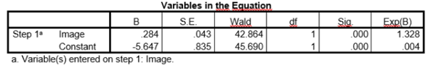
In a study concerning the smoking behavior amongst adolescents, a logistic regression analysis is conducted to check the effect of the image of smoking (Image) on smoking behavior (Smoking).

Image: to what degree the young adult thinks smoking is perceived as “cool”. The variable image is measured on a scale from 10 to 30, in which higher scores indicate that smoking is perceived as cooler.

Smoking: whether or not the adolescent smokes.

0 = the adolescent is a non-smoker
1 = the adolescent is a smoker

Below you can find part of the output the researchers retrieved.

First, write down the estimated regression model.

\(Logit(Smoking = 1) = -5.65 + 0.28*Image\)

What is the probability that an adolescent with a score of 15 on image smokes?

Take a look at the regression coefficient.

Imagine that one’s score on Image will increase from 15 to 16.

To what degree will the logit and odds change?

And what can you conclude about the increase in probability?

The logit increases with 0.284. So −1.387+0.284=−1.103

The odds increase with a factor 1.328. So, the odds become 0.25×1.328=0.332

By just looking at the output, it is unclear what exactly will happen with the probability. We DO know that the probability will increase because the logits and the odds increase.

If we would calculate the probability by hand, we would see that the probability increases with 0.05.

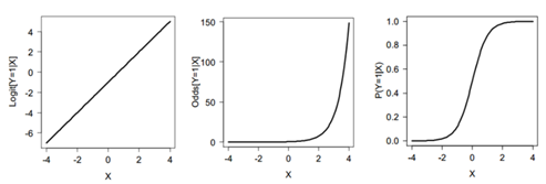
As you can see, the logit follows a linear function, the odds follow an exponential function, and probability follows a logistic function (perhaps less clear from the example but see the graphs below for an illustration). It is nice to work with a linear model (i.e., work with the logits), but from an interpretation point of view odds and probabilities are nicer to work with.

15.2 Logistic Regression

Today we will study whether the probability to pass a Statistics course depends on exam fear and the math grade obtained in high school (prior math ability).

Open LAS BE LR.sav.

In the table below you find the variables included in this fictional data set.

We want to study the following research question:

Does the probability of passing the statistics exam depend on exam stress and math ability?

To answer this question, we first need to dichotomize the dependent variable. This is an unusual step, because dichotomizing variables loses information! Still, for the purpose of the present exercise, we will do so. We will create the new dependent variable Passed (0 = fail, 1 = pass), where a 5.5 or higher counts as a pass. Use the following steps:

Navigate to Transform → Recode into different variables. Select GradeStats as input variable and use Passed as the name for the new recoded variable. Do not forget to click on CHANGE. Click on Old and new values and specify the recoding in such a way that all grades of 5.5 or higher will get the new value 1 and all grades lower than 5.5 (i.e., all other grades) the value 0. Paste and run the syntax. Go to variable view and specify the value labels.

Obtain the frequency distribution for Passed (via Analyze –> Descriptive Statistics –> Frequencies).

What percentage of students passed? %

We will use logistic regression to study the effect of exam stress and math ability on the probability to pass. Take the following steps:

Navigate to Analyze –> Regression –> Binary logistic regression Select Passed as dependent variable and ExamStress and Math as independent variables (in SPSS called “covariates”). Paste and run the syntax.

Inspect the output corresponding to Block 1. Take a look at the table “Variables in the Equation”.

What would be good description of the effects on the sample level? (i.e., what the effect of ExamStress and Math on the probability to pass looks like).

Turns out Exam Stress has a negative effect on the probability to pass (controlled for Math grade), and Math a positive effect (controlled for Exam Stress).

What is the value of the regression coefficient for the variable Exam Stress?

Give a detailed interpretation of this number.

If we would increase one unit in Exam Stress the logits to pass the exam will decrease with 0.025, while keeping the variable Math constant.

True or false: The independent variables Math and Exam Stress together have a significant effect on the probability to pass.

When we inspect the model test, we see that, together, Exam Stress and Math grade have a significant effect on the probability to pass, χ2(2) = 81.043, p < .001.

Second, carry out the significance tests for the individual predictors as well.

True or false: There is a significant effect of Math on the probability to pass, controlled for Exam stress.

True or false: There is a significant effect of Exam stress on the probability to pass, controlled for Math.

When we inspect the separate regression coefficients together, we see that:

Controlled for Exam stress, Math grade has a significant effect on the probability to pass, χ2(1)=54.500, p<.001. Controlled for Math grade, Exam stress has no significant effect on the probability to pass, χ2(1)=0.040, p=.841.

15.3 Logistic Regression with Categorical Predictor

Now, we will carry out a logistic regression analysis to study whether the probability to pass can be predicted from the amount of preparation (Preparation), controlled for prior math ability (Math).

But… the variable Preparation is a nominal (categorical) variable. Use dummy coding to include it in the model. The variable Preparation has three categories. Create all three dummy variables!

Take the following approach to carry out the analysis.

Navigate to Analyze –> Regression –> Binary Logistic

Select Math as covariate.

Select the dummies for Preparation as covariates. At this stage, use “only reading the book” as the reference group.

Paste and run the syntax.

Take a look at the table Variables in the Equation.

Inspect the estimated regression coefficients. Consider the results on the sample level, ignoring inferential statistics for now.

Which group has the highest estimated probability to pass?

Which group has the lowest estimated probability to pass (controlled for math ability)?

Write down the full model equation, filling in the values of coefficients. Then check your answer.

\(logit_{passed} = -5.833 + .300*D_{exercises} + .946*D_{both} + .999 * Math\)

Controlled for Math Grade, what is the difference in predicted odds between people who only read the book and people who read the book and made the exercises?

Take the exponent of the regression coefficient for the dummy for people who read the book and made the exercises (see table).

By hand, calculate the probability that the third person in the file (respID=3) passes the exam.

Imagine that you do not know whether this person passed the exam or not.

True or false: Based on your answer in the previous step and using a decision threshold of .5, you would predict this student to pass.

SPSS can easily calculate the probability to pass.

Either use the visual interface:

Click on the SAVE button in the menu for logistic regression.

Select Probabilities under the header Predicted Values.

Click on continue.

Or add this line of code to your model:

  /SAVE=PRED

SPSS adds a new variable to the data file, which gives the predicted probability for each person. Check whether you calculated the predicted probability for person 3 correctly.

Imagine that we would have used this model to predict the probability to pass for the students in this sample before they even made the exam. Use a decision threshold of .5 to classify students as those likely to pass vs fail.

Out of all students that were classified as “pass”, which proportion actually failed?

Of the 370 students who were predicted to pass, 52 failed the exam (.141). As you can see, the model is not completely flawless in making predictions.

What is worse in your opinion? Incorrectly predicting that students will pass (when they end up failing), or incorrectly predicting that students will fail (when they end up passing)? Why?

If you chose a different decision criteria to predict passing - say .7, what would happen to the proportion of students that were classified as “pass”, but actually failed?

15.4 Hierarchical Logistic Regression

In this assignment we will compare the following two models against each other.

Model1: \(Logit(Pass) = b0+b1∗Math\)
Model2: \(Logit(Pass) = b0+b1∗Math+b2∗ExamStress+b3∗Evaluation\)

Later on, we want to carry out a model comparison test to check whether the larger model predicts the probability of passing the exam better than the smaller model.

What would be the regression df for the model comparison test, in which we compare the larger model 2 to the smaller model 1?

Now we will carry out the model comparison test. Take the following steps.

Navigate to Analyze -> Regression -> Binary Logistic

Select Math as predictor (covariates).

Click on Next (upper right); we can now indicate which block of predictors we like to add in addition to the variables added in the first model.

Enter ExamStress and Evaluation as predictors (covariates).

Paste and run the syntax.

Inspect the output. SPSS organizes the output in three blocks. The results in Block 0 refer to the null model without any predictors. Note that this null model also exists when you use the “Linear Regression” interface, but it’s not featured in the output.

Block 1 refers to the results of Model 1 and Block to the results of Model 2.

Take a look at the results of the model comparison test.

What test statistic is used to compare nested logistic regression models?

What is the value of the appropriate test statistic for comparing models 1 and 2?

True or false: Adding predictors ExamStress and Evaluation lead to significantly better predictions, compared to a model with only high school math grade as predictor.