Probability refers to the likelihood or chance of an outcome occurring in a random experiment. It is defined as the proportion of times that a particular outcome is expected to occur if the experiment is repeated an infinite number of times.
A random experiment is a process with multiple potential outcomes that could theoretically be repeated under similar conditions. For example, flipping a coin is a random experiment, and before flipping the coin, the outcome is a random experiment with a probability of getting heads or tails of 50% each. Once the coin is flipped, the outcome becomes fixed (the opposite of random), resulting in either heads or tails.
In a way, when you draw samples from a population and observe the values of particular variables (e.g., country of origin, height, age), you are performing random experiments. That means that, like with any random experiment, the values you are likely to observe also follow certain probability distributions. Discrete random variables have a finite or countable number of possible outcomes, such as the outcome of a coin toss. On the other hand, continuous random variables, such as the height of individuals, have an infinite number of possible outcomes.
For discrete (categorical) variables, we use discrete frequency and probability distributions, which summarize the observations and probabilities of each possible outcome, respectively. These distributions can be represented using frequency distributions, contingency tables, or bar charts.
Frequency distributions summarize observed outcomes in a sample. For example, a frequency distribution can tell us the proportion of Dutch students in a class or the number of times a particular number was rolled on a die.
Contingency tables (also called crosstables) are used to describe the join frequency distribution, and possibly relationship, between two categorical variables. They show the frequencies of different combinations of values for the two variables.
We can use frequency distributions to estimate the probabilities of observing those outcomes in the future. To calculate probabilities from frequencies, we can use different approaches depending on the type of probability distribution we want. In general, dividing frequencies by the total number of observations (grand total) gives us probabilities. In contingency tables, marginal probability distributions are obtained by dividing the marginal totals (row sums or column sums) by the grand total, which provides us with a probability distribution for each separate variable. Conditional probability distributions are derived by dividing a specific row or column by the row- or column total (marginal total), and tells us the probabilities of one variable given a specific value of the other variable.
In continuous probability distributions, the possible outcomes are infinite and described by a continuous function. One common example is the normal distribution, also known as the bell curve. It is a symmetric distribution that extends from negative infinity to positive infinity, and it is characterized by two parameters: its mean (average) and standard deviation (measure of dispersion). The square of the standard deviation is called the variance.
The standard normal distribution, also known as the Z-distribution, is a standardized version of the normal distribution, rescaled to have a mean of 0 and a standard deviation of 1. Standardizing normal distributions allows us to calculate probabilities more easily using standard normal distribution tables or calculators. We can then convert these probabilities back to the original units if needed.
Probability distributions can be used as models to describe/approximate the distribution of real data. Behind the scenes, we do this any time we describe the distribution of scores on a variable using its mean and standard deviation. While we often assumpe that variables are normally distributed, that assumption is not always accurate. For example, depression symptoms do not follow a normal distribution: Most people score near-zero on depression symptoms, and few people have higher scores (but these are also not normally distributed). In such cases of violations of the assumption of normality, the mean and standard deviation are not very informative. You may use other descriptive statistics, consider different probability distributions (outside the scope of this course), or discuss the limitations of the assumption of normality.
In conclusion, probability distributions provide a way to represent the probabilities associated with different outcomes of a random variable, whether discrete or continuous. By using probability distributions, we can report descriptive statistics, calculate probabilities, and make predictions about future observations.
6.1 Lecture
VIDEO ERRATA: from 10:10 - 10:50 I talk about the probability of Being Dutch and Having a Tattoo, but I’m calculating the probability of Being Dutch and Not Having a Tattoo (I misread the column labels).
6.2 Formative Test
A formative test helps you assess your progress in the course, and helps you address any blind spots in your understanding of the material. If you get a question wrong, you will receive a hint on how to improve your understanding of the material.
Complete the formative test ideally after you’ve seen the lecture, but before the lecture meeting in which we can discuss any topics that need more attention
Question 1
An HR advisor is looking for new employees for LEGO. He thinks it is important for them to be creative. Creativity is normally distributed in the population, with a mean of 180 and a standard deviation of 25. A higher score indicates higher creativity. The advisor only wants to select applicants that belong to the 0.015 proportion of most creative people. What cut-off/boundary score for creativity should the HR advisor use?
Question 2
What is probability?
Question 3
What is a random experiment?
Question 4
What are discrete random variables?
Question 5
What information is contained in a frequency distribution?
Question 6
What is the standard normal distribution?
Question 7
A researcher is interested in the relationship between movie watched and popcorn consumption. She counts the number of people who consume popcorn during a movie, and whether they have watched Mean Girls or not. The results are presented in the table below this quiz. What is P(Popcorn|Mean Girls), rounded to 3 decimal places?
Question 1
Find the Z-score that matches a right tail probability of .015 and calculate \((Z*25) + 180\)
Question 2
(The frequentist definition of) probability builds upon the idea that you could theoretically repeat the random experiment many times and calculate the proportion of times a given outcome is observed
Question 3
A random experiment is a process with multiple potential outcomes that could theoretically be repeated many times under similar conditions.
Question 4
Discrete random variables have a finite (=discrete) or countable number of possible outcomes.
Question 5
Frequency distributions are used to summarize observed outcomes in a sample.
Question 6
The standard normal distribution is a standardized version of the normal distribution with a mean of 0 and a standard deviation of 1.
Question 7
The question is about the conditional probability of having popcorn given that (|) someone watched mean girls; divide the 151 pp who match this description by the total number of people who watched mean girls.
6.2.0.1 Popcorn consumption Table
Popcorn consumption
Yes
No
Total
Movie type
Mean Girls
151
90
241
Other
1678
2130
3808
Total
1829
2220
4049
6.3 Tutorial
6.3.1 Normal Distribution
In this assignment you will practice with the normal distribution.
The normal distribution deserves special attention as it is commonly used in statistics for the social sciences. The normal distribution was already derived in the 18 century by DeMoivre, Adrian, and also Gauss*, and since then it played a central role in statistics. More importantly, many attributes in the social sciences are by close approximation normally distributed, as was first discovered by Quetelet. Hence, the normal distribution has great empirical relevance, which comes in handy for our research!
For that reason, the normal distribution is sometimes referred to as a Gaussian curve.
Before we start, the concept of a random variable needs to be introduced first. A random variable is a numerical outcome of a chance experiment.
For example, a random variable is the number of pips when throwing two dice (here the chance experiment is throwing two dice). Also, the proportion of girls in a random sample of 10 children is a random variable (here the chance experiment is the random selection of 10 children).
We also distinguish between continuous and discrete (categorical) random variables.
A continuous variable can take on infinitely many values. For example, the height of a person is a continuous variable. Take any two persons of different height, and we can always find a third person in between. Discrete variables can take on only particular values. For example, the number of correct of correct answers when a person blindly guesses all the answers is a discrete random variable.
if you want to know, see for example Wikipedia
Normal distributions are distributions for continuous random variables.
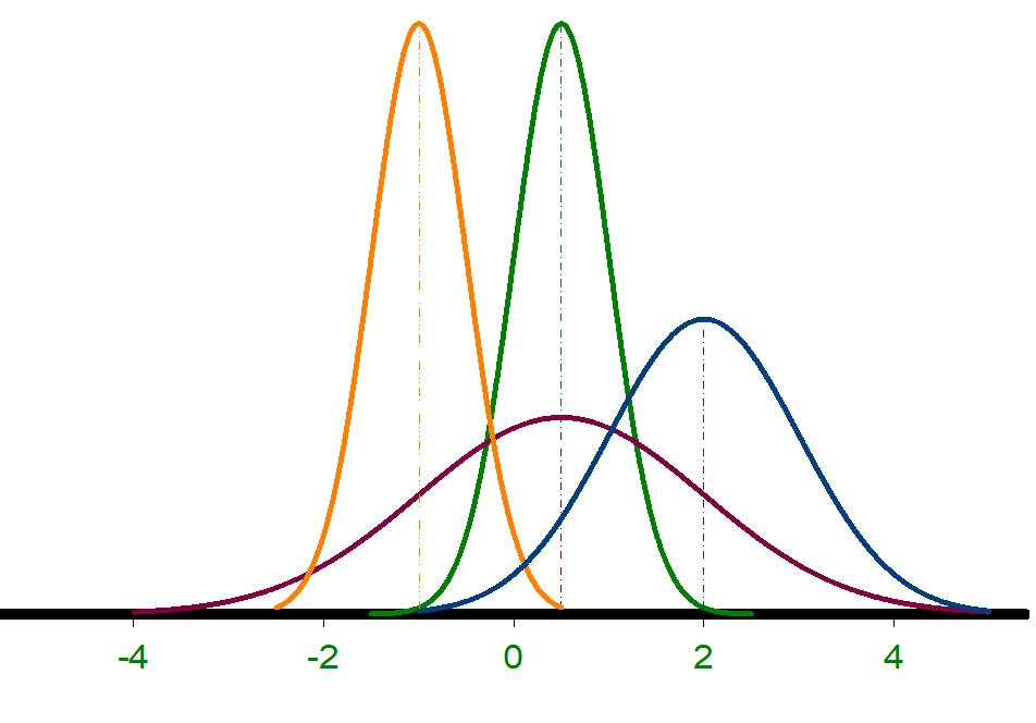
Let’s first have another look at different examples of normal distributions:
Dist.
\(\mu\)
\(\sigma\)
1
–1.0
0.5
2
0.5
0.5
3
0.5
1.5
4
2.0
1.0
Inspection of the graphs of the bell-shape distributions shows that it is a symmetric distribution. We also see that the distributions differ in location (the point on the x-axis where it reaches its maximum) and the spread. In other words, the distribution is characterized by two parameters: the mean and standard deviation. The mean is denoted by the Greek letter \(\mu\) (pronounced as “moo”) and standard deviation is denoted by the Greek letter \(\sigma\) (pronounced as “sigma”).
Compare the distributions and see how the parameters determine the location (mean) and spread (standard deviation).
6.3.1.1 Quiz
Correctly complete the sentence below by filling in the gaps:
Given the example “A student guesses the correct answer to 10 multiple choice questions with four answer categories each” the random experiment is and the random variable is .
Are the following random variables discrete or continuous?
Number of heads in 10 throws with a fair coin is continuous.
Time by train from Tilburg to Eindhoven is continuous.
The number of correct answers on a test is continuous.
The mean height in a random sample is continuous.
The average number of correct answers in a random sample of 100 students is continuous.
If the standard deviation (SD) increases, the distribution becomes
6.3.1.2 “The Empirical Rules”
As a first step we may consider some practical rules for working with the normal distribution, the so called “empirical rules”. In particular, if a random variable is normally distributed the following empirical rules apply:
68% of the values lie within one standard deviation from the mean. 95% of the values lie within two standard deviations from the mean.
If we know that a variable is normally distributed, we can also compute probabilities of certain outcomes, so called events. For example, if we know that the scores on a test are normally distributed, we may want to know the probability that a randomly selected person has a score above a certain cut-off (i.e., satisfies a certain selection criterion).
In the next few steps, you will practice on how to compute probabilities under the normal distribution. To do so, we have to be able to work with the standard normal distribution (Z-distribution) and accompanying tables.
6.3.1.3 Quiz
Complete the following sentences:
IQ scores are normally distributed with mean 100 and an SD of 15. This means that 95% of the persons in the population has an IQ in between and .
Students loan after completing the bachelor is normally distributed with mean 1500 Euros and an SD of 150. This means that 68% of the students ends up with a loan between and .
What is the mean of the standard normal distribution?
What is the SD of the standard normal distribution?
6.3.1.4 Calculating probabilities
For the next series of exercises you need to use a Z-table or calculator (e.g., Excel, Google Sheets, R online, or the Z-table in this GitBook, Appendix B).
We have seen that probabilities are related to the area under the curve. This means that for continuous variables we can only find the probability that the outcome falls within a certain interval. For example, the time to complete a task is more than 10 minutes; the IQ is in between 70 and 90.
Note that there may be different ways to get to the correct answer.
Numerical Examples
6.3.1.5 Quiz
Consider a continuous variable X, which is normally distributed with \(X \sim(\mu = 30, \sigma = 4)\).
Compute the following probabilities:
P(X>36.8):
P(X<24):
P(X<35):
P(28<X<34):
P(X>36.8):
Transform X into Z: (36.8 − 30)/4 = 1.7
Read Upper Tail Area for Z = 1.7, which equals 0.0446
Conclusion: P(X>36.8)= 0.0446.
P(X<24):
Transform X into Z: (24 − 30)/4 = -1.5
Because the Z-distribution is symmetric, we know that P(Z<−1.5) is equal to P(Z>1.5). The latter probability can be found in the Z-table, which is 0.0668. This is also the probability we are looking for.
Conclusion: P(X<24) = 0.0668.
P(X<35):
The probability we are looking for equals 1− P(X>35). Thus, we first need P(X>35).
Compute corresponding Z-value: Z = = 1.25.
Look for the upper tail area in the Z-table: P(Z>1.25) = .1056.
Thus, the area we are looking for is 1 − .1056 = .8944
Conclusion: P(Z<35) = 0.89444
P(28<X<34):
Remark: there are different ways to come the answer. So the answer below is just one of few possibilities.
We need the area under curve between 28 and 34. This area equals 1 minus the tail areas; that is, P(28<X<34) = 1 − P(X<28) − P(X>34)
Lets start with P(X>34). First compute Z= = 1. Via the Z-table we find P(Z>1)= .1587.
Now determine P(X<28). First compute Z= = −0.5. Via the Z-table we find P(Z<−0.5) = P(Z>0.5) = .3085.
Hence, we have 1 − 0.1587 − 0.3085 = 0.5328
Conclusion: P(28<X<34) = 0.5328.
Students are looking for a new roommate. They read in an article that the time people spend under the shower is in the population normally distributed with mean of 10 and SD of 8 (measured in minutes). Suppose they randomly select a person as their new roommate.
What is the probability that this randomly selected person will spend more than 20 minutes under the shower?
Suppose “confidence in society” is measured on a continuous scale from 0 (no confidence at all) to 100 (highly confident). Also suppose that confidence is normally distributed in the population with mean 52.6 and SD of 12. One speaks of low confidence if the score falls below 43.
What percentage of the population has low confidence?
The scores on a test for aggressive behavior are normally distributed with mean 50 and SD of 10. The test is used to select police officers. In particular, only police officers with scores between 42 and 62 qualify for the job as they are not too aggressive and not too friendly either.
What percentage of the population qualifies as police officer?
Let X denote time people spend under the shower. We want to know the probability that the person showers for more than 20 minutes; that is, P(X>20) given \(\mu\) = 10 and \(\sigma\) = 8.
Compute Z value: (20 −10)/8 =1.25. Hence, we need P(Z>1.25); that is, the area beyond Z = 1.25.
Via the Z-table (look in the column labelled C) we find: P(Z>1.25) = .1056.
Conclusion: the probability that a random selected person will shower more than 20 minutes is 0.106 (about 11%).
Let X stands for the confidence level. X is normally distributed with mean = 52.6 and SD = 12. We need P(X<43). That is, we need the area under the curve to the left of 43.
First, transform to Z-scores: X=43 => Z = (43 −52.6)/12 = −0.8. Thus, we need P(Z<−.8).
The left-tail areas are not shown in the Z-table. Therefore, to find the area, we will first look for the area in the other tail; that is, we will look for P(Z>0.8) in the Z-table. The probability equals 0.2119. Because the distribution is symmetric, the left tail area is also 0.2119. This gives us the answer.
Conclusion: about 21.2% in the population has low confidence in society.
Let X be the test scores. We need to compute P(42<X<62). This area can not be directly found in the Z-table, so we have to take some additional steps. First, because the whole area under the curve is 1, we can say that the area we are looking for is equal to 1 minus the areas in the tail; thus, 1 − P(X<42) − P(X>62). These latter probabilities can be read from the Z-table!
Determine the tail areas: because the distribution is symmetric, we have P(Z<−0.8)=P(Z>0.8). The latter can found in Z-table, which equals .2119. Probability P(Z>1.2) can be directly read from the Z-table, which is .1151.
Hence, 1 − .2119 − .1151 = 1−.327 = .673.
Conclusion: 67.3% of the population qualifies as police officer.
Suppose the time to complete a certain task is normally distributed with mean 8.6 and standard deviation (SD) of 3.5.
What is the probability that a randomly selected person needs more than 11.4 minutes to complete the task?
Again, suppose the time to complete a task is normally distributed with mean 8.6 and standard deviation of 3.5.
Complete the sentence:
“95% of the participants completes the task within 1.6 and minutes.”
Scores on a selection test are normally distributed with a mean of 500 and a standard deviation of 50. A person qualifies for the job if they score between 480 and 580.
What is the probability that a randomly selected person will qualify for the job?
An IT company is looking for new programmers. To qualify for the job the programmers need to score high on conscientiousness. Therefore, the job applicants need to complete the Conscientiousness scale from the NEO-PI-R (a popular personality inventory for the Big Five personality traits*) as part of the selection procedure. Research has shown that in the population the scores on the scale are normally distributed with a mean of 133.4 and SD of 18.3. To qualify for the job, the conscientiousness of the programmer needs to be among the highest 20% in the population.
What cut-off should the company use to select new personnel? Round to a whole number.
The Big Five is a popular model for personality; see Wikipedia for more info on the Big Five.
Question 1:
Transform X into Z: (11.4 -8.6)/3.5 = 0.8
Read Upper Tail Area for Z = 0.8, which equals 0.2119
Conclusion: P(X>36.8)= 0.212
Question 2:
95% of the participants completes the task within 1.6 and 15.6 minutes. You can use the empirical rule that 95% of the observations falls within 2SDs from the mean. Thus, 95% of the observations lies within 8.6−2×3.5 and 8.6+2×3.5
And 8.6+2×3.5 = 15.6
Question 3:
We need P(480<X<580). This probability equals 1 − P(X<480) − P(X>580).
So the final answer equals: 1−0.3446−0.0548=0.6006 (0.601 when rounded at three decimal places).
Question 4:
To get to the correct answer, these are the steps: - First find the Z-value that marks the highest 20%. This value equals 0.84. - Then compute the corresponding cut-off on the X-scale: X = 0.84×18.3 + 133.4 = 148.772 - Rounded to the nearest integer equals 149.
6.3.2 Missing Values
For this assignment, and also later assignments, we will use a (real) data set on Type D personality and several background characteristics (age, gender, and education level (7 ordered levels)).
Type D personality is defined as the tendency towards negative affectivity (NA) (e.g., worry, irritability, gloom) and social inhibition (SI) (e.g., reticence and a lack of self-assurance). Theory suggests that Type D individuals have poorer health outcomes.
Type D is measured with the DS14 scale. The DS14 consists of 14 items, 7 measuring NA and 7 items measuring SI. Answers are given on a five point scale (scored 0 through 4).
see also Type D personality on Wikipedia.
Open the data file TypeDDataSSC.sav in SPSS. The data file contains the scores on the DS14 items measuring Type D as well as the background variables for 80 respondents.
Go to the variable view. The content of the items are given under labels and it is indicated whether the item measures NA or SI.
6.3.2.1 Quiz
Is the first item in the DS14 an indicator of NA or SI?
Go to the data view in SPSS and inspect the data.
Do you see any missings?
What is the valid N of the variable age?
How many system missings do we have on gender?
6.3.2.2 Recoding missing values
Remember that Empty cells are called system missings. There are reasons to use user-specified missing codes instead; for example, this allows you to keep track of reasons for missingness (which enables you to report more comprehensively on your missing data).
So, for this exercise we will define a user-missing code for the missing values. Missing code is number that a researcher uses to designate that the value is missing. The code must be chosen such that it cannot be confused with actual scores. For example, for age the missing code can be 999, because 999 is an impossible age.
Now, we will first define missings for age.
Go to the data view; look at the values of age and whenever the value is missing fill in 999. (In total three persons had a missing on age; so you have to fill in 999 three times).
Go to the variable view. We have to define the missing code under missing. Click on the cell and […], and SPSS opens a new window. Define 999 as missing code.
In the previous step we filled in the missing codes manually. For a small data set this is okay, but for large data sets (say thousands of persons on many variables) this would be problematic.
In the next few steps we will see how we can define the missings more easily.
To do so, we will use the function recode in SPSS. We will first apply the recoding to gender.
Before going into the recoding, let’s first look at the frequency table for gender.
You may already have this output from answering the Quiz.
6.3.2.3 Recode into Same Variables
Replacing user missing values with a missing code using the recode option works as follows:
Navigate to Transform > Recode into the same variables. SPSS opens a new window.
Select gender as the variable to be recoded.
Click on Old and New Values. SPSS opens a new window. In this window we can specify the recoding. In our case we want to recode System Missing into 999. So, choose “system missing” as old Value, and specify 999 as new value, and click on Add below. (See the more info section below for the SPSS specifications.)
Click on Continue, and click on OK. SPSS now replaced system missing by 999. Go to the data view and verify that SPSS filled in 999 at the empty places.
Go to the variable view and specify 999 as the user missing code for gender. (In the same way as you did for age).
Compute the frequency table for gender again.
Verify that all “system missings” are now reported as “user missings” instead.
In the previous step we only recoded the missings for gender, but we could do that for all variables. It is most convenient to use a code that can be used for all variables. In this case we can use 999 as the missing code for all variables, it’s easy because we can apply this recoding to all variables at once. Just follow the same steps as before, but now select all variables to recode.
Run the recode command for all variables.
Verify in the data file that SPSS replaced all system missings by 999.
Now we also have to specify in the variable view that 999 is the missing codes for all variables. We already changed it for age and gender. To do the same thing for other variables is easy; you can just use copy-paste! Click on Missing for gender, click on the right mouse button, choose copy. Go to the next variable, click on the right mouse button, and with paste you can define the missings for other variables.
Tip: If you like shortcuts: you can also click on missing, type Ctrl C, and then use Ctrl V to copy the information about the missings.
So, we specified the missing codes, but we also want to know for each respondent how many missings values he or she had. In other words, for each participant we want to count the number of missings. Participants with too many missings may be excluded from further analysis. Counting the number of missings per person can also be easily accomplished in SPSS.
Transform > Count Values within Cases. SPSS opens a new window. Specify the name of the target variable (e.g., CountMiss); this is the name of a new variable that gives the number of missings. You may also give the variable a label, say: “Number of Missings”.
Select all variables.
Click on Define Values. SPSS opens a new window. Select System or User Missing at the left and click on add. Click on continue than OK.
SPSS will now create a new variable that shows how many missings there are for each person on the variables selected in the list.
Go to the data view and verify that SPSS added a new variable (i.e., a new column with values) named CountMiss.
6.3.2.4 Quiz
Compute the frequency table for the third DS14 item. How many missing values do we have on this item?
How many missings does person 8 have, using the variable CountMiss?
Compute the frequency table for CountMiss.
What is the maximum number of missings for the participants in this dataset?
How many participants have this many missings?
How many participants have at least one missing value?
Make sure you save the data file including the variable with the number of missings. We will use it in the next assignment. `
6.3.3 Select Cases and Split File
In this assignment we will take a closer look at selecting cases and how to do analyses for subgroups.
6.3.3.1 Selecting Cases
In the previous assignment we have seen that some respondents had one or more missing values. Suppose we want to discard these persons in the analysis, which means that for all the remaining analyses we only want to include participants with no missings. This method of handling missing data is called listwise deletion, and it is generally considered bad practice - but it’s also easy, so we will teach it in this course. More advanced courses cover expert methods of handling missing data.
Proceed as follows:
Data > Select cases. SPSS opens a new window.
Chose “If condition is satisfied” and chose ‘if’. SPSS opens a new window again.
Specify the condition CountMiss = 0 to select cases with no missings.
Make sure that the output is specified as “Filter out unselected cases”. Click on OK.
Go to the data view.
Verify that SPSS crossed out cases with one or more missings.
Verify that SPSS added a new variable labelled ‘filter_$’. This is filter variable indicating who is included in the analyses (value = 1) or not (value is 0). If you remove the filter variable, SPSS will use all cases again.
6.3.3.2 Quiz
What is the mean for the variable age of the selected group?
What is the valid sample size for that mean?
Now, run the selection procedue again, but remove the incomplete cases from the data file.
Proceed as follows:
Data > Select cases Choose “Delete Unselected Cases” under output. Click OK. Verify that the incomplete cases are removed.
Because you have modified the data, it is prudent to save the new file under a different name (e.g., TypeD_selection.sav). Use this file with only the complete cases (i.e., TypeD_selection.sav) for the remaining steps.
6.3.3.3 Split File
Sometimes we want to do analyses for subgroups, especially when exploring the data for the first time. For example, we may want to have the descriptive statistics for males and females separately. One way to do this is to use the Split File option. With this option you can tell SPSS that you want to have tables for each subgroup separately.
Let’s see how it works!
Proceed as follows:
Via menu follow Data > split file. SPSS opens a new window.
Choose ‘Compare Groups’ and choose gender as the variable for Groups Based on.
Click OK.
Important: Notice no output appears and no changes are made to the data. This makes sense because we haven’t asked SPSS to generate any output nor to make changes in the data. Yet, SPSS now knows that he has to produce tables for males and females separately once we ask to generate output.
To undo the split file, proceed as follows.
Data > Split file Choose Analyze all cases, do not create groups. Click OK. SPSS now no longer produces the output per group.
6.3.3.4 Quiz
Have SPSS compute the mean and SD for age.
How many women are there in the sample? What is the mean age of men in the sample? What is the mean age of women in the sample?
One of the variables is Education Level. It is an ordinal variable with 7 levels, score 1 represents the lowest level of education, and score 7 the highest.
Compute the mean age per level of education.
For which education level was the mean age highest?
What was the value of the mean age for this education level?
6.3.4 Recode and Compute
For this assignment we will continue with the data on Type D and the selection of complete cases.
Before you start, make sure that the Split File option is disabled.
In practice, you often have to do some data handling before you can actually start doing analyses. For example by coding missing values, or you may have questionnaire data for which some of the questions are formulated contra-indicative and therefore should be reverse coded. Another reason would be that you may have to compute the total score (e.g., sum or average) for a set of questions.
In this assignment we will practice some basic data handling skills.
6.3.4.1 Reverse Scoring Contra Indicative Items
If you read the item labels, you will see that the first two SI items (items DS14_1 and DS14_3 in the scale) are contra indicative. This means that for these items higher scores reflect low SI, while for other items higher scores reflect high SI. Therefore, the responses to these items should be recoded first to make sure that all items are scored in the same direction. To do so, we will create new variables that reflect the recoded items. Proceed as follows:
Transform > Recode into different Variables
Choose DS14_1 as the Numerical Variable to be recoded
Specify a name for the output variable (say DS14_1R)
Give a label, say: “SI item 1 (recoded)”
Click on change
Do not close the window yet, but continue to the next step…
To recode, we have to specify the Old Values and New values. Reverse scoring of the DS14 items means that
old value 0 -> new value 4
old value 1 -> new value 3
old value 2 -> new value 2 (*)
old value 3 -> new value 1
old value 4 -> new value 0
(*) You may think this line is superfluous but for the recoding in SPSS you need to specify for every possible value a recoded new value, even if the values remains the same.
Specify the old and new values. Each time you specified old and new values click on ADD such that the recoding scheme appears in the little dialog.
6.3.5 Using Syntax
To ensure that others can see exactly how you got from raw data to the final dataset used for analysis, it is essential to keep a complete record of any changes made to the data. This is also why we previously argued that you should not overwrite a datafile after altering it.
Up until now, we ran the analyses by “click-and-point” via the menu. This is a good starting point to explore the software SPSS, but it is not good practice for professional use because there’s no record of what you did to the data in order to get your result.
NOTE: For all your portfolio assignments, providing syntax is mandatory so I can grade what you DID, not just what you reported!
To keep a record of changes made to your data, you can prepare a script that contains all instructions for the analysis instead. By evaluating this script on the data, you should consistently get the same results.
6.3.5.1 Why syntax?
Using syntax is important for several reasons:
First, efficiency: it makes life easier. Once you have the syntax, you can easily redo the whole analysis without going through all the points-and-clicks again.
Second, communication: When you work together on research projects, it is important that you exactly understand the analyses that were done, even if you didn’t do the analyses yourself. By using syntax, all team members can see what has been done and how.
Third, documentation & data management: As a researcher you are responsible for data storage and management (!). This not only includes storage of data, but also documentation of the all the steps and analyses you did to come to your results (e.g., handling missing values, detection of outlying values). Ideally, you should provide the materials such that other researchers can easily replicate your analyses starting from the raw data file. Working with SPSS syntax is a great way to do so.
Fourth, necessity: some statistical procedures are only available via SPSS syntax (e.g., simple effects analysis in MANOVA).
6.3.5.2 Help!
You don’t need to memorize the commands by heart. SPSS offers help functions. If you highlight the command (e.g., statistics) and click on the button with the paper and the question mark in the top menu. SPSS opens a help file.
Use the help function to modify the syntax such that SPSS produces a table that also reports the range (e.g., the difference between the largest and smallest value).
6.3.5.3 How to use syntax
There are two ways to use syntax. The first is to create an empty syntax script via File -> New -> Syntax, and then start adding the code from scratch. You can either write the code as text, or create it via SPSS’ various dialog windows. For this course, we recommend using the dialogs:
In any dialog window, click “Paste” instead of “OK”.
A new window opens (or existing window comes into focus) with a script file (or “syntax” file). The instructions for the requested analysis are added at the bottom of this file.
Select all instructions you wish to execute, and press the green “Play” button.
You can re-organize this script file, adding, or removing operations or changing their order. Keep it nice and organized!
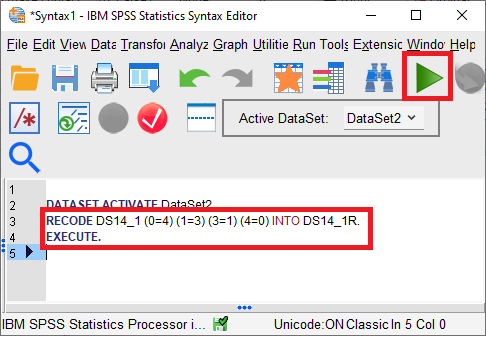
Syntax for recoding
Select the highlighted lines and press the green “Play” button. Verify in the data view that SPSS added a new variable (i.e., new column) with the recoded values for Item 1.
Syntax is also useful because it may be more straightforward than the graphical interface. For example, the recode syntax above took a lot of pointing and clicking to get:
RECODE DS14_1 (0=4) (1=3) (3=1) (4=0) INTO DS14_1R.
EXECUTE.
For recoding more variables, we can copy-paste these instructions and change the variable names.
For example, to recode DS14_3 in the same way as you did the recoding for DS14_1 we would write:
RECODE DS14_1 (0=4) (1=3) (3=1) (4=0) INTO DS14_1R.
RECODE DS14_3 (0=4) (1=3) (3=1) (4=0) INTO DS14_3R.
EXECUTE.
When working with syntax, it is highly recommended to add comments as reminders to your future self of the purpose of each step in the script. These comments should clarify the syntax and give general information (e.g., when was the syntax last modified, who did the modifications, etc.).
Comments are text lines that start with an * and ends with a dot. Comments are printed in grey.
REMARK: the dot at the end of your text line is really important. If you do not add it, your syntax will run work properly!
Add comments including the following information:
When was the syntax made?
Who made syntax?
What does the syntax do?
For example (CJ is short for Caspar J. Van Lissa):
* CJ: This script also recodes Likert scales with integer values.
COMPUTE DS14_1R = 4-DS14_1.
COMPUTE DS14_3R = 4-DS14_3.
EXECUTE.
After including the comments, run the complete syntax including the comment line (by selecting and running it, or via top menu Run > All).
If the syntax runs correctly, the comments were correctly included.
6.3.5.5 Compute Variable
For the analyses we are not interested in the single item scores but in the summed scores. Because the DS14 contains two subscales (consult the item labels to see to which subscale the item belongs), we want to compute the summed scores for the NA and SI items separately.
Let’s first do this for NA. Proceed as follows:
Transform > Compute variable. SPSS opens a new window.
Choose a name for the target variable, say: NAtotal.
Under numerical expression you have to say what you want to compute. In this case the sum of the NA items, which is DS14_2 + DS14_4 + … etc. So, select the first item to be summed from the list at the left, type +, select the next item you want to add, and so on. Make sure that you only add up the NA items (in the variable view you can see which items measure NA and which measure SI).
Click Paste, and run the code.
Alternatively, copy-paste this syntax, complete it and run it:
Compute the frequency table for the recoded DS14_3 item.
What percentage of the respondents had the highest score on this item?
What is the mean of NAtotal?
Compute the mean of NAtotal for men and women separately. For which group is the mean highest? (Hint: Use the skills you’ve learned in the previous assignments).
Compute the total scores for SI. Make sure you use the reverse scored items for items 1 and 3 to compute the total score (this implies you have to leave the original item 1 and 3 out).