3  Bivariate Descriptive Statistics

In the previous chapter, we covered univariate (= single variable) descriptive statistics. In this chapter, we introduce the first bivariate (= two variables) descriptive statistics. Let’s take stock of the road so far, and set a goal for where we want to go. Last week, we ended with the variance. The variance is a statistic that tells us, on average, how much people’s scores deviate from the mean. Today we will move into bivariate descriptive statistics. We will learn about the covariance, which tells us: If someone’s score on one variable deviates positively from the mean, is their score on another variable also likely to deviate positively from the mean? We will also learn about the correlation, which tells us: How strong is the association between two variables, and is it positive or negative?

In this chapter, we will talk about two hypothetical variables, X and Y. In your mind, you can substitute any two variables you like; for example, X = hours studied, Y = grade obtained, or X = extraversion, Y = number of friends.

Before arriving at the correlation coefficient, statisticians often begin with covariance—a preliminary measure of how two variables vary together. Covariance reflects direction: it is positive when high values of X accompany high values of Y, and negative when they move in opposite directions. However, its numerical value is not directly interpretable because it is tied to the units of the measurement. A covariance expressed in centimeters and kilograms will differ from one computed in meters and pounds, even if the underlying association remains unchanged. As a result, covariance cannot meaningfully convey the strength of a relationship—only whether the variables tend to move in the same or opposite directions.

It provides a concise summary of the association between pairs of scores across individuals. For example, a researcher might retrieve each student’s high school GPA (a measure of academic performance) and pair it with their family’s annual income. The goal is to determine whether higher grades tend to correspond with higher income. In correlational studies, each individual contributes two measurements, commonly referred to as X and Y forming the foundation for analysis.

The correlation coefficient is a statistic that quantifies the strength and direction of association between two variables. It tells us the degree to which two variables move together. One way to think of the correlation coefficient is as a bivariate (= two variables) descriptive statistic.

To explore this relationship visually, researchers often rely on scatter plots. In a scatter plot, X values appear along the horizontal axis and Y values along the vertical. Each point on the plot corresponds to one participant’s pair of scores. These plots allow immediate detection of linear trends, and outliers—patterns that may remain obscured when examining data in purely numerical or tabular form.

3.1 Covariance

The word “covariance” means: varying, or moving, together. Let’s have a look at mock data from five students on hours studied and final grade obtained:

set.seed(2)
grads <- data.frame(
  Hours = round(runif(5, 2, 20))
)
grads$Grade <- round(scales::rescale(.7*grads$Hours + rnorm(5), to = c(1, 10)))
knitr::kable(grads)

Hours	Grade
5	3
15	9
12	6
5	1
19	10

We can visualize these data using a “scatterplot”; a simple graph where each observation is shown as a dot with X-coordinate determined by their value on the X variable (Hours), and Y-coordinate determined by the Y variable (Grade):

library(ggplot2)
ggplot(grads, aes(x = Hours, y = Grade)) + geom_point() + theme_bw()

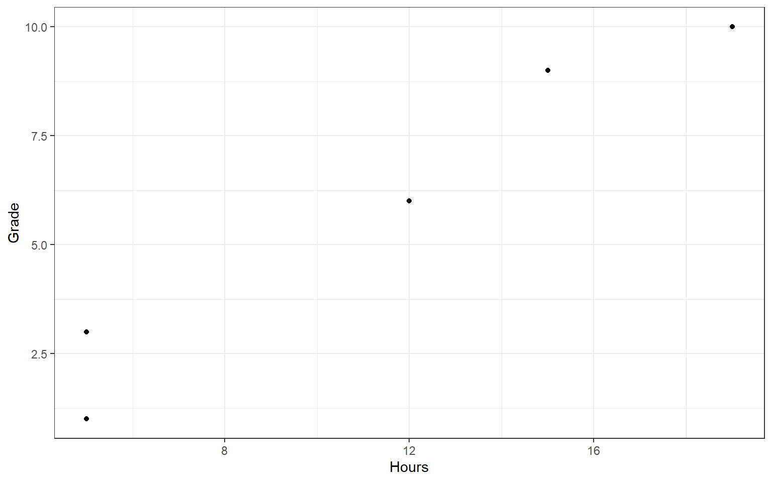
Notice that, if you squint, it appears like there might be some pattern in the data: more hours studied tends to go hand in hand with a higher grade. There might be a positive association between these variables! In the next sections, we go about quantifying this association numerically, step by step.

3.1.1 Sum of Products (SP)

The first stage in quantifying the association between two variables is to compute the sum of products of deviations (SP). The SP is similar to the sum of squares (SS), but whereas the SS captures the variability of one variable, the SP measures how two variables vary together.

To calculate the SP, take the following steps:

3.1.1.1 Step 1: Calculate the variables’ means

Take the mean of each column (bold in the table below):

library(kableExtra)
mns <- grads
mns[] <- lapply(mns, as.character)
mns <- rbind(mns, colMeans(grads))
names(mns) <- c("X", "Y")
kable(mns) |>
  kable_styling() |>
  row_spec(nrow(mns),bold=T,hline_after = T)

X	Y
5	3
15	9
12	6
5	1
19	10
11.2	5.8

3.1.1.2 Step 2: Calculate Deviations

For each variable, calculate the deviations by subtracting the mean from the observed scores:

library(kableExtra)
devs <- grads
devs <- cbind(devs, sweep(devs, 2, colMeans(devs)))
names(devs) <- c("X", "Y", "X-mean(X)", "Y-mean(Y)")
kable(devs)

X	Y	X-mean(X)	Y-mean(Y)
5	3	-6.2	-2.8
15	9	3.8	3.2
12	6	0.8	0.2
5	1	-6.2	-4.8
19	10	7.8	4.2

3.1.1.3 Step 3: Multiply Deviations

If we were to calculate the SS, we would now square the deviations and add them up in each column. To get the SP, instead of squaring the deviations - we multiply them across variables. Note that if the deviations for both variables have the same sign, then this will give a positive result (positive times positive is positive, and negative times negative is positive too). Moreover, if the deviations from both variables are high, the product will be a high number too. So the SP tends to be a large positive number if high positive (or negative) deviations on one variable go hand in hand with high positive (or negative) deviations on the other variable.

prods <- devs
prods <- cbind(prods, apply(devs[, 3:4], 1, prod))
names(prods)[5] <- "Product"
kable(prods)

X	Y	X-mean(X)	Y-mean(Y)	Product
5	3	-6.2	-2.8	17.36
15	9	3.8	3.2	12.16
12	6	0.8	0.2	0.16
5	1	-6.2	-4.8	29.76
19	10	7.8	4.2	32.76

Now, we calculate the SP just by taking the sum of the column of products: 92.2.

Note that if the SP is positive, then there is a positive association between the variables; if it is negative, there is a negative association. In this case, the association is positive.

Here is a formula describing what we just did: we took the sum \(\Sigma\) of the product \(()()\) of the deviations of X from the mean of X, \(X-\bar{X}\) times the deviations of Y from the mean of Y, \(Y-\bar{Y}\):

\[ SP = \sum \bigl(X - \bar{X}\bigr)\bigl(Y - \bar{Y}\bigr) \]

3.1.2 Covariance

To get the covariance from the sum of products, we divide by the sample size, so in this case, \(\frac{92.2}{5}\).

Another way to think about this is: we standardize the SP by the sample size \(n\). This gives us the “average co-deviation” per participant. That number is called the covariance.

If the covariance is positive, there is a positive association between the two variables. If it is negative, there is a negative association.

But how strong is the association? It is hard to say, because the size of the covariance depends on the units and scale of the two variables involved.

3.2 Correlation

To answer the question of how strong the association is, we must standardize the covariance to drop the units of both variables. This gives us the so-called Pearson correlation coefficient (r). Specifically, the covariance is divided by the product of the standard deviations of X and Y. This standardization results in a number between -1 and +1, where 0 means no association, -1 means perfect negative association, and +1 means perfect positive association. This number, the correlation coefficient, tells us both the direction (-/+) and strength (value) of association between two variables. Because the correlation coefficients is unit-free, or standardized, it can also be compared across variables measured on different scales and across studies.

3.3 Limitations

While correlation coefficients are useful, they must be interpreted with care.

To illustrate the limitations of correlations, the statistician Anscombe (1973) created four data sets with identical correlation coefficients, \(r = 0.82\). When plotting the data, however, it becomes clear that the correlation coefficient can only be meaningfully interpreted for the first dataset (figure a below).

plts <- lapply(1:4, function(i){
  df <- anscombe[, paste0(c("x", "y"), i)]
  names(df) <- c("X", "Y")

  ggplot(df, aes(x = X, y = Y)) + geom_point(shape = 21, size = 3, fill = "orange") + theme_linedraw()
})
ggpubr::ggarrange(plotlist = plts, ncol = 2, nrow = 2, labels = "auto")

Figure 3.1: Anscombe’s quartet, 1973

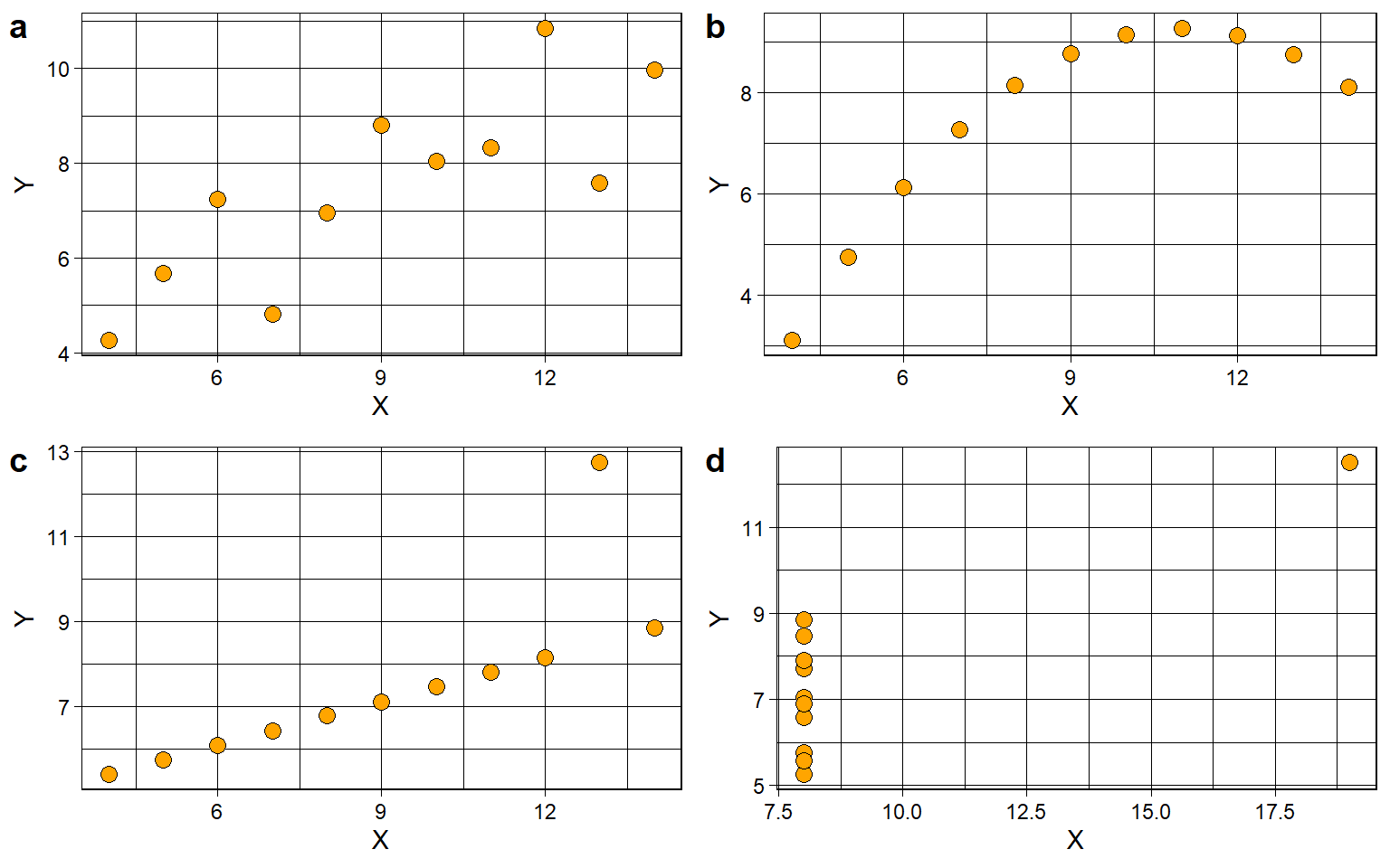
The first and most important limitation is that, Pearson’s correlation coefficient only meaningfully captures linear associations, or: patterns that look like a straight line. Note that figure a in Figure 3.1 shows such a linear pattern of association; the correlation coefficient of \(r = .82\) tells us that there is a strong - but not perfect - positive association.

Figure b in Figure 3.1 , on the other hand, shows a perfect non-linear association. All dots are perfectly in line; the line is just not straight. This illustrates that Pearson’s correlation coefficient is not suited for capturing non-linear patterns, even if a strong relationship exists in another form.

Figure c shows a correlation of \(r = 1\) for most of the points - but one outlier brings it down to \(r = .82\).

Figure d shows no association at all for most of the points (they all have the same value for X, and if X does not vary, it cannot covary/correlate with Y) - but a single outlier makes it look like there is a strong correlation..

Secondly, these plots illustrate that outliers can have a disproportionate impact. In figures c and d, a single extreme observation artificially deflates (c) or inflates (d) the correlation coefficient, potentially leading to misleading conclusions.

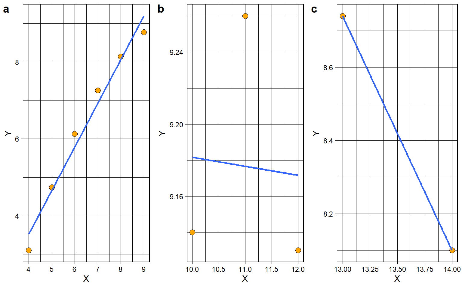
Thirdly, a restricted range of scores can obscure or distort relationships. For example, if you were to examine the pattern in figure b of Figure 3.1 for values of X between [4, 9], you would conclude that \(r = 0.99\), or near perfect positive correlation. If you examined the same pattern for values of X between (0, 13), you would conclude that \(r = -0.07\), or near-zero. If you examined the same pattern for values of X between [13, 20), you would conclude that \(r = -1.00\), or perfect negative correlation. Figure Figure 3.2 below zooms into the pattern from figure b, by restricting the range of variable X into three segments:

df <- anscombe[, paste0(c("x", "y"), 2)]
names(df) <- c("X", "Y")
p1 <- ggplot(df[df$X <= 9, ], aes(x = X, y = Y)) + geom_point(shape = 21, size = 3, fill = "orange") + theme_linedraw()+ geom_smooth(method = "lm", se = FALSE)
p2 <- ggplot(df[df$X > 9 & df$X < 13, ], aes(x = X, y = Y)) + geom_point(shape = 21, size = 3, fill = "orange") + theme_linedraw() + geom_smooth(method = "lm", se = FALSE)
p3 <- ggplot(df[df$X >= 13, ], aes(x = X, y = Y)) + geom_point(shape = 21, size = 3, fill = "orange") + theme_linedraw() + geom_smooth(method = "lm", se = FALSE)
ggpubr::ggarrange(p1,p2,p3, ncol = 3, nrow = 1, labels = "auto")

`geom_smooth()` using formula = 'y ~ x'
`geom_smooth()` using formula = 'y ~ x'
`geom_smooth()` using formula = 'y ~ x'

Figure 3.2: Zooming in on panel b of Anscombe’s quartet, restricting the range of X

Restriction of range can easily happen in real life. For example, if your sample only consists of university students, you will probably havce restriction of range on IQ.

Finally, you may have heard the phrase correlation does not imply causation. Observing a strong association between two variables does not mean that one causes the other. In general, it is not possible to conclude causality from statistics: causality is an assumption, which can be either supported by a theory, or by a particular methodology. In a randomized controlled experiment, participants are randomly assigned to receive either a treatment or control condition. Thus, any differences between the two groups should be due to the experimental treatment, or random chance. We will revisit the topic of causality later.

Anscombe’s quartet is a good illustration of the limitations of causality, and also demonstrates the value of visually inspecting your data (including with scatter plots) before interpreting any statistics.

3.4 Summary

In summary, covariance offers an initial metric for gauging whether two variables tend to vary in the same or opposite direction. However, because its magnitude depends on the measurement units of the variables involved, it cannot be directly interpreted in terms of strength. The Pearson correlation coefficient (r) addresses this limitation by standardizing the covariance, yielding a unit-free statistic bounded between –1 and +1. This standardized measure expresses both the direction and strength of a linear relationship, enabling meaningful comparisons across contexts. Nevertheless, interpreting correlations requires caution, particularly with respect to restricted sampling ranges, the influence of outliers, and the fundamental distinction between correlation and causation.

4 Formative Test

This short quiz checks your grasp of Chapter 3 – Covariance & Correlation.
Work through it after you’ve studied the lecture slides (and before the next live session) so we can focus on anything that still feels uncertain. Each incorrect answer reveals a hint that sends you back to the exact slide or numerical example you need.

add_mcs("ch3_formative_corrected.csv")

::: {.webex-check .webex-box}

**Question 1**

question <div class='webex-radiogroup' id='radio_HGAVIPDKFI'><label><input type="radio" autocomplete="off" name="radio_HGAVIPDKFI" value=""></input> <span>B</span></label><label><input type="radio" autocomplete="off" name="radio_HGAVIPDKFI" value=""></input> <span>A</span></label><label><input type="radio" autocomplete="off" name="radio_HGAVIPDKFI" value=""></input> <span>C</span></label><label><input type="radio" autocomplete="off" name="radio_HGAVIPDKFI" value="answer"></input> <span>answer</span></label><label><input type="radio" autocomplete="off" name="radio_HGAVIPDKFI" value=""></input> <span>D</span></label></div>


**Question 2**

A covariance of +120 cm·kg tells you… <div class='webex-radiogroup' id='radio_WHMFBWRCTC'><label><input type="radio" autocomplete="off" name="radio_WHMFBWRCTC" value=""></input> <span>The units have been standardised</span></label><label><input type="radio" autocomplete="off" name="radio_WHMFBWRCTC" value=""></input> <span>A perfect linear trend</span></label><label><input type="radio" autocomplete="off" name="radio_WHMFBWRCTC" value=""></input> <span>120 % of Y variance explained</span></label><label><input type="radio" autocomplete="off" name="radio_WHMFBWRCTC" value="answer"></input> <span>X and Y tend to rise together</span></label><label><input type="radio" autocomplete="off" name="radio_WHMFBWRCTC" value=""></input> <span>X and Y tend to rise together</span></label></div>


**Question 3**

If the covariance between study hours and stress level is negative, what does that imply? <div class='webex-radiogroup' id='radio_ARHDMEBUVM'><label><input type="radio" autocomplete="off" name="radio_ARHDMEBUVM" value="answer"></input> <span>Longer study → lower stress</span></label><label><input type="radio" autocomplete="off" name="radio_ARHDMEBUVM" value=""></input> <span>Longer study → lower stress</span></label><label><input type="radio" autocomplete="off" name="radio_ARHDMEBUVM" value=""></input> <span>Units are incomparable</span></label><label><input type="radio" autocomplete="off" name="radio_ARHDMEBUVM" value=""></input> <span>No relationship</span></label><label><input type="radio" autocomplete="off" name="radio_ARHDMEBUVM" value=""></input> <span>Longer study → higher stress</span></label></div>


**Question 4**

Which statement about covariance magnitude is true? <div class='webex-radiogroup' id='radio_DIJORFVSOM'><label><input type="radio" autocomplete="off" name="radio_DIJORFVSOM" value=""></input> <span>It ranges only from –1 to +1</span></label><label><input type="radio" autocomplete="off" name="radio_DIJORFVSOM" value=""></input> <span>It equals the regression slope</span></label><label><input type="radio" autocomplete="off" name="radio_DIJORFVSOM" value=""></input> <span>A larger value always means a stronger relationship</span></label><label><input type="radio" autocomplete="off" name="radio_DIJORFVSOM" value=""></input> <span>Its size depends on measurement units</span></label><label><input type="radio" autocomplete="off" name="radio_DIJORFVSOM" value="answer"></input> <span>Its size depends on measurement units</span></label></div>


**Question 5**

Converting temperatures from Celsius to Fahrenheit will make the covariance between temperature and ice-cream sales… <div class='webex-radiogroup' id='radio_MQEFQZIUXO'><label><input type="radio" autocomplete="off" name="radio_MQEFQZIUXO" value=""></input> <span>Increase by a constant factor</span></label><label><input type="radio" autocomplete="off" name="radio_MQEFQZIUXO" value=""></input> <span>Switch sign</span></label><label><input type="radio" autocomplete="off" name="radio_MQEFQZIUXO" value=""></input> <span>Stay exactly the same</span></label><label><input type="radio" autocomplete="off" name="radio_MQEFQZIUXO" value="answer"></input> <span>Increase by a constant factor</span></label><label><input type="radio" autocomplete="off" name="radio_MQEFQZIUXO" value=""></input> <span>Become unit‑free</span></label></div>


**Question 6**

Pearson’s r is best described as… <div class='webex-radiogroup' id='radio_UKIOJNEKQL'><label><input type="radio" autocomplete="off" name="radio_UKIOJNEKQL" value=""></input> <span>Mean of X and Y combined</span></label><label><input type="radio" autocomplete="off" name="radio_UKIOJNEKQL" value="answer"></input> <span>Standardised (unit-free) covariance</span></label><label><input type="radio" autocomplete="off" name="radio_UKIOJNEKQL" value=""></input> <span>Raw measure of joint variability</span></label><label><input type="radio" autocomplete="off" name="radio_UKIOJNEKQL" value=""></input> <span>Ratio of two variances</span></label><label><input type="radio" autocomplete="off" name="radio_UKIOJNEKQL" value=""></input> <span>Standardised (unit-free) covariance</span></label></div>


**Question 7**

If r = 0, we can conclude that… <div class='webex-radiogroup' id='radio_TADVXYFWNG'><label><input type="radio" autocomplete="off" name="radio_TADVXYFWNG" value="answer"></input> <span>No linear relationship is present</span></label><label><input type="radio" autocomplete="off" name="radio_TADVXYFWNG" value=""></input> <span>X causes Y</span></label><label><input type="radio" autocomplete="off" name="radio_TADVXYFWNG" value=""></input> <span>X and Y are unrelated in every way</span></label><label><input type="radio" autocomplete="off" name="radio_TADVXYFWNG" value=""></input> <span>The data contain no outliers</span></label><label><input type="radio" autocomplete="off" name="radio_TADVXYFWNG" value=""></input> <span>No linear relationship is present</span></label></div>


**Question 8**

A positive covariance but r ≈ 0.05 usually indicates that… <div class='webex-radiogroup' id='radio_IEZCAGNYKE'><label><input type="radio" autocomplete="off" name="radio_IEZCAGNYKE" value=""></input> <span>The variables move together only slightly</span></label><label><input type="radio" autocomplete="off" name="radio_IEZCAGNYKE" value="answer"></input> <span>The variables move together only slightly</span></label><label><input type="radio" autocomplete="off" name="radio_IEZCAGNYKE" value=""></input> <span>Units have been standardised</span></label><label><input type="radio" autocomplete="off" name="radio_IEZCAGNYKE" value=""></input> <span>Data range is restricted to zero</span></label><label><input type="radio" autocomplete="off" name="radio_IEZCAGNYKE" value=""></input> <span>The relationship is strong</span></label></div>


**Question 9**

Which scatter‑plot feature primarily determines the sign of covariance (and r)? <div class='webex-radiogroup' id='radio_LBZTIQWSEH'><label><input type="radio" autocomplete="off" name="radio_LBZTIQWSEH" value=""></input> <span>Overall slope direction</span></label><label><input type="radio" autocomplete="off" name="radio_LBZTIQWSEH" value=""></input> <span>Point density</span></label><label><input type="radio" autocomplete="off" name="radio_LBZTIQWSEH" value=""></input> <span>Sample size</span></label><label><input type="radio" autocomplete="off" name="radio_LBZTIQWSEH" value=""></input> <span>Presence of a mode</span></label><label><input type="radio" autocomplete="off" name="radio_LBZTIQWSEH" value="answer"></input> <span>Overall slope direction</span></label></div>


**Question 10**

You multiply every X score by 10 but leave Y unchanged. What happens? <div class='webex-radiogroup' id='radio_HMQEPDGXSH'><label><input type="radio" autocomplete="off" name="radio_HMQEPDGXSH" value=""></input> <span>Covariance × 10; r unchanged</span></label><label><input type="radio" autocomplete="off" name="radio_HMQEPDGXSH" value=""></input> <span>Both covariance and r unchanged</span></label><label><input type="radio" autocomplete="off" name="radio_HMQEPDGXSH" value=""></input> <span>Covariance unchanged; r × 10</span></label><label><input type="radio" autocomplete="off" name="radio_HMQEPDGXSH" value=""></input> <span>Covariance × 10; r × 10</span></label><label><input type="radio" autocomplete="off" name="radio_HMQEPDGXSH" value="answer"></input> <span>Covariance × 10; r unchanged</span></label></div>


**Question 11**

A covariance of 0 implies that… <div class='webex-radiogroup' id='radio_TJRTMRLVPV'><label><input type="radio" autocomplete="off" name="radio_TJRTMRLVPV" value=""></input> <span>X and Y are unrelated in every way</span></label><label><input type="radio" autocomplete="off" name="radio_TJRTMRLVPV" value="answer"></input> <span>Their linear relationship (r) is 0</span></label><label><input type="radio" autocomplete="off" name="radio_TJRTMRLVPV" value=""></input> <span>Their linear relationship (r) is 0</span></label><label><input type="radio" autocomplete="off" name="radio_TJRTMRLVPV" value=""></input> <span>They have opposite scales</span></label><label><input type="radio" autocomplete="off" name="radio_TJRTMRLVPV" value=""></input> <span>X causes Z</span></label></div>


**Question 12**

Two variables show r = 0.85. Which conclusion is justified? <div class='webex-radiogroup' id='radio_ORROVCURTK'><label><input type="radio" autocomplete="off" name="radio_ORROVCURTK" value=""></input> <span>X and Y are associated; causal direction unknown</span></label><label><input type="radio" autocomplete="off" name="radio_ORROVCURTK" value=""></input> <span>Y causes X</span></label><label><input type="radio" autocomplete="off" name="radio_ORROVCURTK" value="answer"></input> <span>X and Y are associated; causal direction unknown</span></label><label><input type="radio" autocomplete="off" name="radio_ORROVCURTK" value=""></input> <span>A third variable is impossible</span></label><label><input type="radio" autocomplete="off" name="radio_ORROVCURTK" value=""></input> <span>X causes Y</span></label></div>


**Question 13**

Analysing data with a restricted range typically makes r… <div class='webex-radiogroup' id='radio_XLKCVYNXFP'><label><input type="radio" autocomplete="off" name="radio_XLKCVYNXFP" value=""></input> <span>Larger in magnitude</span></label><label><input type="radio" autocomplete="off" name="radio_XLKCVYNXFP" value=""></input> <span>Smaller in magnitude</span></label><label><input type="radio" autocomplete="off" name="radio_XLKCVYNXFP" value=""></input> <span>Exactly zero</span></label><label><input type="radio" autocomplete="off" name="radio_XLKCVYNXFP" value=""></input> <span>Change sign</span></label><label><input type="radio" autocomplete="off" name="radio_XLKCVYNXFP" value="answer"></input> <span>Smaller in magnitude</span></label></div>


**Question 14**

An extreme outlier that follows the overall trend will most likely… <div class='webex-radiogroup' id='radio_PFXFMKRLCS'><label><input type="radio" autocomplete="off" name="radio_PFXFMKRLCS" value="answer"></input> <span>Inflate the magnitude of r</span></label><label><input type="radio" autocomplete="off" name="radio_PFXFMKRLCS" value=""></input> <span>Inflate the magnitude of r</span></label><label><input type="radio" autocomplete="off" name="radio_PFXFMKRLCS" value=""></input> <span>Drive r toward zero</span></label><label><input type="radio" autocomplete="off" name="radio_PFXFMKRLCS" value=""></input> <span>Remove measurement error</span></label><label><input type="radio" autocomplete="off" name="radio_PFXFMKRLCS" value=""></input> <span>Make covariance negative</span></label></div>


**Question 15**

A coefficient of determination (r²) of 0.49 means that… <div class='webex-radiogroup' id='radio_HWDADJCQNI'><label><input type="radio" autocomplete="off" name="radio_HWDADJCQNI" value=""></input> <span>49 % of Y variance is explained by X</span></label><label><input type="radio" autocomplete="off" name="radio_HWDADJCQNI" value=""></input> <span>49 % of X variance is explained by Y</span></label><label><input type="radio" autocomplete="off" name="radio_HWDADJCQNI" value=""></input> <span>The correlation is −0.70</span></label><label><input type="radio" autocomplete="off" name="radio_HWDADJCQNI" value="answer"></input> <span>49 % of Y variance is explained by X</span></label><label><input type="radio" autocomplete="off" name="radio_HWDADJCQNI" value=""></input> <span>Covariance is unit‑free</span></label></div>


**Question 16**

After converting both X and Y to z‑scores, the covariance of those z‑variables equals… <div class='webex-radiogroup' id='radio_ZKRKUCTKUW'><label><input type="radio" autocomplete="off" name="radio_ZKRKUCTKUW" value="answer"></input> <span>Pearson’s r</span></label><label><input type="radio" autocomplete="off" name="radio_ZKRKUCTKUW" value=""></input> <span>Pearson’s r</span></label><label><input type="radio" autocomplete="off" name="radio_ZKRKUCTKUW" value=""></input> <span>Their geometric mean</span></label><label><input type="radio" autocomplete="off" name="radio_ZKRKUCTKUW" value=""></input> <span>Always zero</span></label><label><input type="radio" autocomplete="off" name="radio_ZKRKUCTKUW" value=""></input> <span>Sample size</span></label></div>


:::


<div class='webex-solution'><button>Show explanations</button>
**Question 1**

explanation

**Question 2**

Positive sign = same-direction movement; magnitude is unit-dependent so strength not directly interpretable.

**Question 3**

Negative covariance means high X pairs with low Y and vice‑versa.

**Question 4**

Rescaling either variable rescales covariance; therefore magnitude alone is not comparable across units.

**Question 5**

Multiplying Celsius by 1.8 and adding 32 rescales covariance by 1.8; adding a constant does not affect it.

**Question 6**

Dividing covariance by the product of SDs removes units and bounds the result between –1 and +1.

**Question 7**

r only detects linear association; other patterns may still exist.

**Question 8**

Small r means weak linear association despite positive sign.

**Question 9**

Positive slope → positive sign; negative slope → negative sign.

**Question 10**

Scaling one variable scales covariance by that factor but leaves r (unit‑free) unchanged.

**Question 11**

Zero covariance means no linear co‑movement; nonlinear links could still exist.

**Question 12**

Correlation quantifies association but cannot establish causality without experimental control.

**Question 13**

Less variability reduces covariance relative to the SDs, shrinking r.

**Question 14**

Trend‑consistent outliers add leverage, increasing |r|.

**Question 15**

r² translates correlation into variance‑explained terms.

**Question 16**

Standardising divides by SDs, so covariance in z‑space equals r.


</div>

5 Tutorial

5.1 Load Data

Open LAS_SocSc_DataLab2.sav (find it in the data folder you downloaded earlier).
The file contains six variables (X1 … X6). You’ll inspect three bivariate relationships.

5.1.1 Plot the pairs

Generate three simple scatterplots:

1. Graphs › Legacy Dialogs › Scatter/Dot ► Simple Scatter
   
2. Pairings & axis order
   • X1 (X-axis) vs X2 (Y-axis)
     
   • X3 (X-axis) vs X4 (Y-axis)
     
   • X5 (X-axis) vs X6 (Y-axis)
     
3. Paste and Run each syntax block.

Describe linearity, direction, and strength for each plot.

“The relationship between X1 and X2 is positive.” TRUE FALSE

“The relationship between X5 and X6 is positive.” TRUE FALSE

“The relationship between X1 and X2 is linear.” TRUE FALSE

“The relationship between X3 and X4 is linear.” TRUE FALSE

Strength of X1–X2:
moderate strong weak zero

Strength of X3–X4:
strong weak zero moderate

Strength of X5–X6:
strong weak zero moderate

5.1.2 Correlation coefficients

Even when the pattern is non-linear it’s useful to see why Pearson r can mislead.

Analyze › Correlate › Bivariate
Select all six variables → OK.

X1–X2 correlation:

X2–X6 correlation:

X3–X4 correlation:

Can we interpret X3–X4’s r at face value?
No, assumption of association violated No, assumption of linearity violated No, assumption of normality violated Yes, otherwise SPSS would give an error

Interpret X5–X6:
Weak negative Moderate negative Weak positive Moderate positive

Take-away: Pearson’s r is good at detecting linear patterns (like X1–X2), but it may be close to zero even when the variables have a strong curved pattern (like X3–X4).

5.2 Correlation – Work Dataset (Work.sav)

Having practiced on simulated data, let’s now apply the same workflow to a real dataset related to the workplace.

File location: data/Work.sav

5.2.1 Why inspect the plot first?

Before trusting Pearson r we check for

• an approximately linear pattern, and
  
• extreme values that could distort the statistic.

Select the correct reason:

To check if the relationship is linear To check if the relationship is positive To check if the relationship is strong enough

5.2.2 Create the scatter-plot

Graphs › Legacy Dialogs › Scatter/Dot → Simple Scatter

• X-axis =scmental (Mental Pressure)
  
• Y-axis =scemoti (Emotional Pressure)

Paste and Run.

The cloud of data points is roughly linear: TRUE FALSE

There are obvious outliers: TRUE FALSE

Approximate strength:

Moderately strong and positive Moderately weak and positive Moderately strong and negative Moderately weak and negative

5.2.3 Compute Pearson r

Analyze › Correlate › Bivariate → (scmental, scemoti) → OK

The correlation coefficient is (2 decimals):

Interpretation:

There is a relationship between mental and emotional pressure. There is no relationship between mental and emotional pressure. We cannot draw a conclusion on whether or not there is a relationship.

Take-away: Mental and emotional pressure show a moderately strong, significant positive relationship—employees who feel more mentally pressured also tend to feel more emotionally pressured.