Chapter 9 Meta-Regression

Conceptually, Meta-Regression does not differ much from a subgroup analysis. In fact, subgroup analyses with more than two groups are nothing more than a meta-regression with categorial covariates. Meta-regression with continuous moderators reveals whether values of this continuous variable are linearly associated with the effect size.
The idea behind meta-regression
In a conventional regression, we specify a model predicting the dependent variable \(y\), across \(_i\) participants, based on their values on \(p\) predictor variables, \(x_{i1} \dots x_{ip}\). The residual error is referred to as \(\epsilon_i\). A standard regression equation therefore looks like this:
\[y_i=\beta_0 + \beta_1x_{1i} + ...+\beta_px_{pi} + \epsilon_i\]
In a meta-regression, we want to estimate the effect size \(\theta\) of several studies \(_k\), as a function of between-studies moderators. There are two sources of heterogeneity: sampling error, \(\epsilon_k\), and between-studies heterogeneity, \(\zeta_k\) so our regression looks like this:
\[\theta_k = \beta_0 + \beta_1x_{1k} + ... + \beta_px_{pk} + \epsilon_k + \zeta_k\]
You might have seen that when estimating the effect size \(\theta_k\) of a study \(k\) in our regression model, there are two extra terms in the equation, \(\epsilon_k\) and \(\zeta_k\). The same terms can also be found in the equation for the random-effects-model in Chapter 4.2. The two terms signify two types of independent errors which cause our regression prediction to be imperfect. The first one, \(\epsilon_k\), is the sampling error through which the effect size of the study deviates from its “true” effect. The second one, \(\zeta_k\), denotes that even the true effect size of the study is only sampled from an overarching distribution of effect sizes (see the Chapter on the Random-Effects-Model for more details). In a fixed-effect-model, we assume that all studies actually share the same true effect size and that the between-study heterogeneity \(\tau^2 = 0\). In this case, we do not consider \(\zeta_k\) in our equation, but only \(\epsilon_k\).
As the equation above has includes fixed effects (the \(\beta\) coefficients) as well as random effects (\(\zeta_k\)), the model used in meta-regression is often called a mixed-effects-model. Mathematically, this model is identical to the mixed-effects-model we described in Chapter 7 where we explained how subgroup analyses work.
Indeed subgroup analyses are nothing else than a meta-regression with a categorical predictor. For meta-regression, these subgroups are then dummy-coded, e.g.
\[ D_k = \{\begin{array}{c}0:ACT \\1:CBT \end{array}\]
\[\hat \theta_k = \theta + \beta x_{k} + D_k \gamma + \epsilon_k + \zeta_k\]
In this case, we assume the same regression line, which is simply “shifted” up or down for the different subgroups \(D_k\).
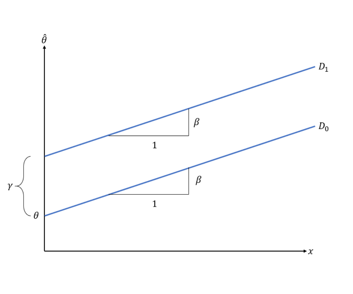
Figure 9.1: Visualisation of a Meta-Regression with dummy-coded categorial predictors
Assessing the fit of a regression model
To evaluate the statistical significance of a predictor, we conduct a t-test of its \(\beta\)-weight.
\[ t=\frac{\beta}{SE_{\beta}}\]
Which provides a \(p\)-value telling us if a variable significantly predicts effect size differences in our regression model.
If we fit a regression model, our aim is to find a model which explains as much as possible of the current variability in effect sizes we find in our data.
In conventional regression, \(R^2\) is commonly used to quantify the percentage of variance in the data explained by the model, as a percentage of total variance (0-100%). As this measure is commonly used, and many researchers know how to to interpret it, we can also calculate a \(R^2\) analog for meta-regression using this formula:
\[R_2=\frac{\hat\tau^2_{REM}-\hat\tau^2_{MEM}}{\hat\tau^2_{REM}}\]
Where \(\hat\tau^2_{REM}\) is the estimated total heterogenetiy based on the random-effects-model and \(\hat\tau^2_{REM}\) the total heterogeneity of our mixed-effects regression model.
NOTE however, that \(R^2\) refers to variance explained in the observed data. The more predictors you add, the better your model will explain the observed data. But this can decrease the generalizability of you model, through a process called overfitting: You’re capturing noise in your dataset, not true effects that exist in the real world.