10.1 Detecting publication bias
Various methods to assess and control for publication bias have been developed, but we will only focus on a few well-established ones here. According to Borenstein et al. (Borenstein et al. 2011). The model behind the most common small-study effects methods has these core assumptions:
- Because they involve large commitment of ressources and time, large studies are likely to get published, weather the results are significant or not
- Moderately sized studies are at greater risk of missing, but with a moderate sample size even moderately sized effects are likely to become significant, which means that only some studies will be missing
- Small studies are at greatest risk for being non-significant, and thus being missing. Only small studies with a very large effect size become significant, and will be found in the published literature.
In accordance with these assumptions, the methods we present here particularly focus on small studies with small effect sizes, and wheather they are missing.
10.1.1 Funnel plots
The best way to visualize whether small studies with small effect sizes are missing is through funnel plots.
We can generate a funnel plot for our m_re meta-analysis output using the funnel() function in metafor:
funnel(m_re, xlab = "Hedges' g")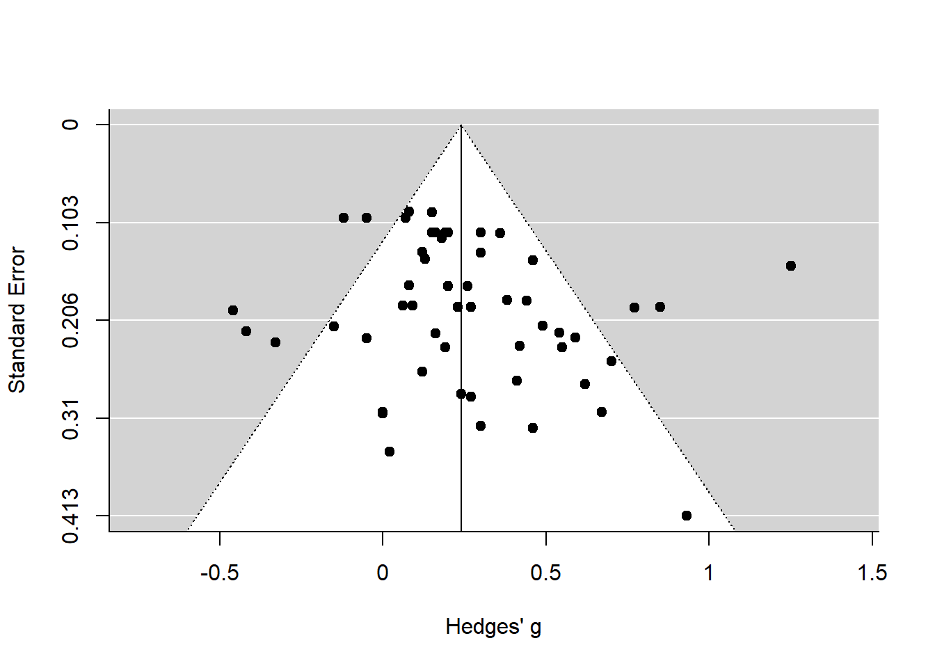
The funnel plot basically consists of a funnel and two axes: the y-axis showing the Standard Error \(SE\) of each study, with larger studies (which have a smaller \(SE\)) plotted on top of the y-axis; and the x-axis showing the effect size of each study.
Given our assumptions, and in the case when there is no publication bias, all studies would lie symmetrically around our pooled effect size (the vertical line in the middle), within the form of the funnel. When publication bias is present, we would assume that the funnel would look asymmetrical, because only the small studies with a large effect size very published, while small studies without a significant, large effect would be missing.
We see from the plot that in the case of our meta-anlysis, there is no obvious publication bias among the smaller studies, but there are a few moderately-sized studies that fall outside of the funnel shape. These are the outliers we investigated earlier.
We can also display the name of each study using the studlab parameter.
10.1.2 Egger’s test
Remember that we can formally test for funnel asymmetry, by predicting the effect size from its standard error. For this, we can simply apply the regtest function to our existing random-effects meta-analysis, and the SE will be used as a predictor:
regtest(m_re)##
## Regression Test for Funnel Plot Asymmetry
##
## model: mixed-effects meta-regression model
## predictor: standard error
##
## test for funnel plot asymmetry: z = 1.0714, p = 0.2840The result is non-significant, so there is no evidence for asymmetry.
10.1.3 Contour-enhanced funnel plots
An even better way to inspect the funnel plot is through contour-enhanced funnel plots, which help to distinguish publication bias from other forms of asymmetry (Peters et al. 2008). Contour-enhanced funnels include colors signifying the significance level into which the effects size of each study falls (p < .05, p < .01, and p < .001). We can plot such funnels using this code:
funnel(m_re, level=c(90, 95, 99), shade=c("white", "gray55", "gray75"), refline=0)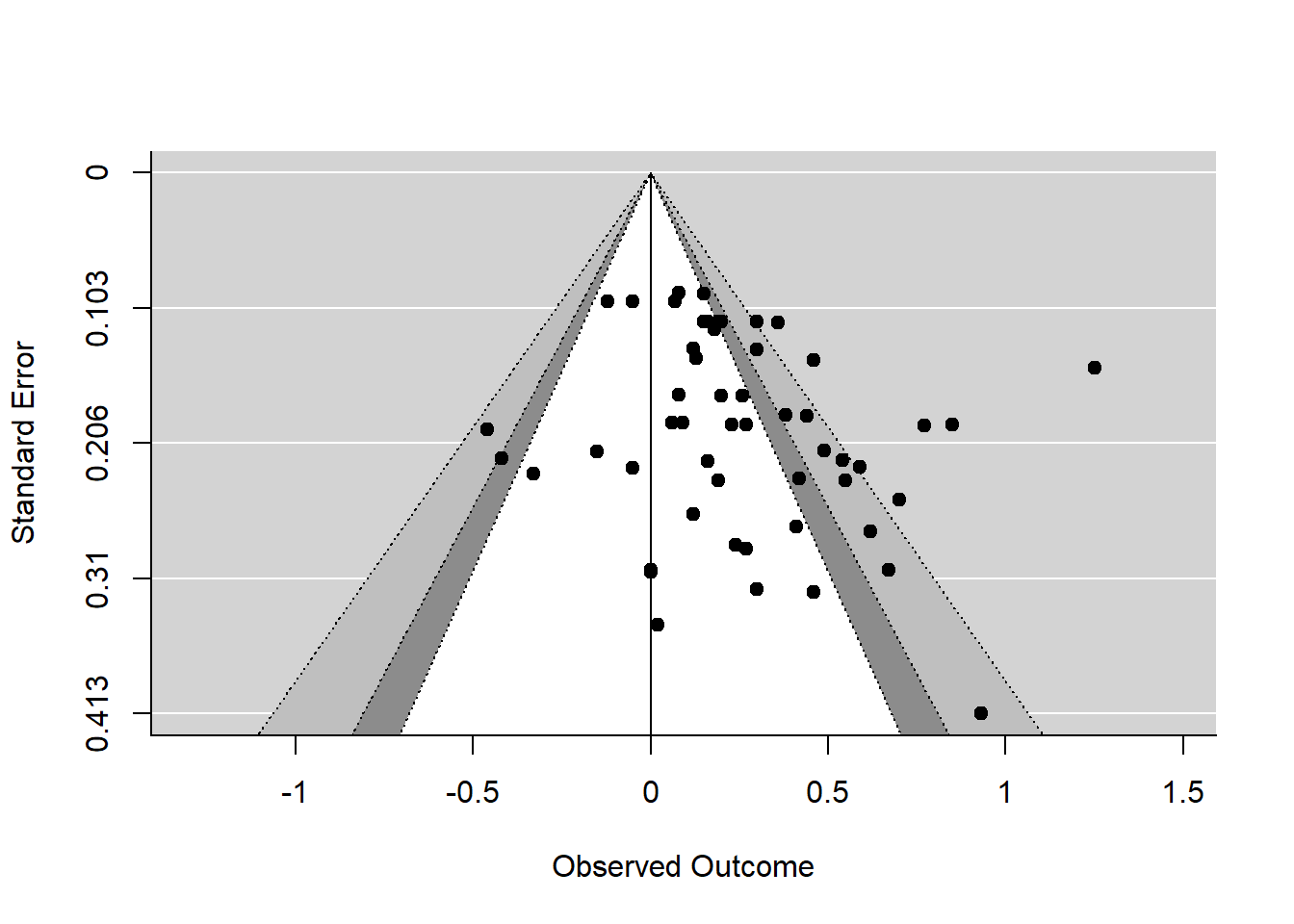
We can see in the plot that while some studies have statistically significant effect sizes (the gray areas), others do not (white background). We see that the significant studies are primarily on the right side of the line.
10.1.4 Testing for funnel plot asymmetry using Egger’s test
Egger’s test for funnel plot asymmetry (Egger et al. 1997) quantifies the funnel plot asymmetry and performs a statistical test:
regtest(m_reg)##
## Regression Test for Funnel Plot Asymmetry
##
## model: mixed-effects meta-regression model
## predictor: standard error
##
## test for funnel plot asymmetry: z = 1.0337, p = 0.3013The function uses regression to test the relationship between the observed effect sizes and the standard error of the effect sizes. If this relationship is significant, that might indicate publication bias. However, asymmetry could have been caused by other reasons than publication bias. In this case, there is no significant asymmetry.
10.1.5 Duval & Tweedie’s trim-and-fill procedure
Duval & Tweedie’s trim-and-fill procedure (Duval and Tweedie 2000) is also based the funnel plot and its symmetry/asymmetry. When Egger’s test is significant, we can use this method to estimate what the actual effect size would be had the “missing” small studies been published. The procedure imputes missing studies into the funnel plot until symmetry is reached again.
The trim-and-fill procedure includes the following five steps (Schwarzer, Carpenter, and Rücker 2015):
- Estimating the number of studies in the outlying part of the funnel plot
- Removing (trimming) these effect sizes and pooling the results with the remaining effect sizes
- This pooled effect is then taken as the center of all effect sizes
- For each trimmed/removed study, a additional study is imputed, mirroring the effect of the study on the left side of the funnel plot
- Pooling the results with the imputed studies and the trimmed studies included
The trim-and-fill-procedure can be performed using the trimfill function in metafor. For this example, we will first introduce some intentional publication bias:
df_bias <- df

# Identify the 20 effect sizes with the smallest effect sizes
small_effects <- order(df_bias$d)[1:20]
# Of these small effect sizes, find the ones with the biggest sampling variance
big_variance <- order(df_bias$vi[small_effects], decreasing = TRUE)
# Delete these studies:
delete_these <- small_effects[big_variance[1:10]]
df_bias <- df_bias[-delete_these, ]
Now, we re-do some of the analyses:
# Fit random-effects model
m_bias <- rma(d, vi, data = df_bias)

# Test for publication bias is now significant:
regtest(m_bias)
##
## Regression Test for Funnel Plot Asymmetry
##
## model: mixed-effects meta-regression model
## predictor: standard error
##
## test for funnel plot asymmetry: z = 2.8682, p = 0.0041# Carry out trim-and-fill analysis
m_taf <- trimfill(m_bias)
m_taf##
## Estimated number of missing studies on the left side: 16 (SE = 4.2698)
##
## Random-Effects Model (k = 62; tau^2 estimator: REML)
##
## tau^2 (estimated amount of total heterogeneity): 0.1127 (SE = 0.0274)
## tau (square root of estimated tau^2 value): 0.3356
## I^2 (total heterogeneity / total variability): 80.45%
## H^2 (total variability / sampling variability): 5.11
##
## Test for Heterogeneity:
## Q(df = 61) = 269.1227, p-val < .0001
##
## Model Results:
##
## estimate se zval pval ci.lb ci.ub
## 0.1480 0.0498 2.9732 0.0029 0.0504 0.2455 **
##
## ---
## Signif. codes: 0 '***' 0.001 '**' 0.01 '*' 0.05 '.' 0.1 ' ' 1We see that the procedure identified and trimmed 16 studies (with 16 added studies)). The overall effect estimated by the procedure is \(g = 0.1480\).
Let’s compare this to our initial results.
m_re$b[1]## [1] 0.2392596The initial pooled effect size was \(g = 0.2393\), which is substantially larger than the bias-corrected effect. In our case, if we assume that publication bias was a problem in the analyses, the trim-and-fill procedure lets us assume that our initial results were overestimated due to publication bias, and the “true” effect when controlling for selective publication might be \(g = 0.1480\) rather than \(g = 0.2394\). Of course, we intentionally introduced the bias in this case.
We can also create funnel plots including the imputed studies:
# Draw funnel plot with missing studies filled in
funnel(m_taf)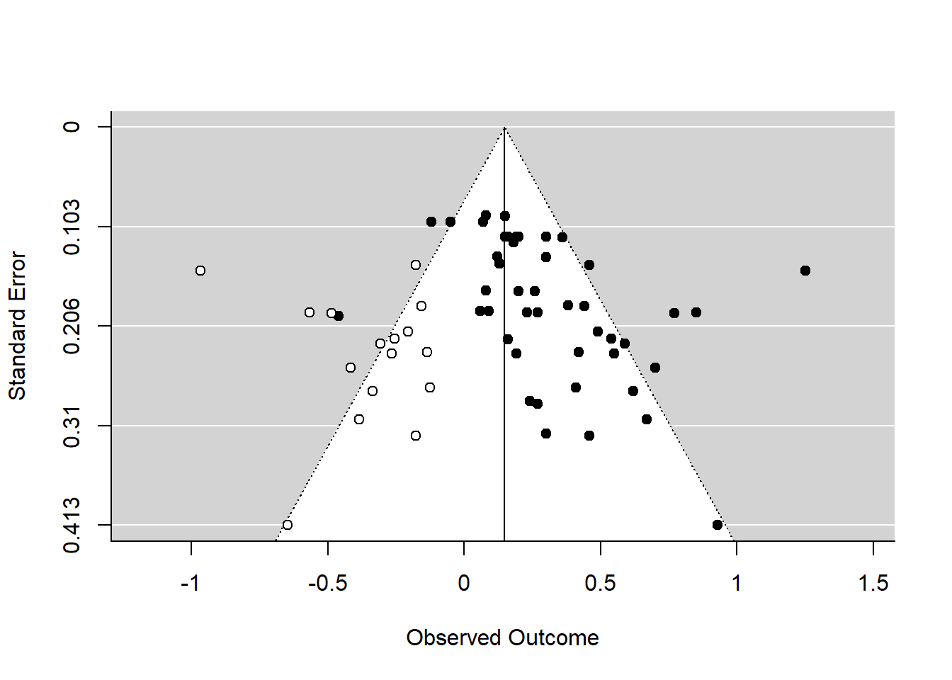
References
Borenstein, Michael, Larry V Hedges, Julian PT Higgins, and Hannah R Rothstein. 2011. Introduction to Meta-Analysis. John Wiley & Sons.
Duval, Sue, and Richard Tweedie. 2000. “Trim and Fill: A Simple Funnel-Plot–Based Method of Testing and Adjusting for Publication Bias in Meta-Analysis.” Biometrics 56 (2). Wiley Online Library: 455–63.
Egger, Matthias, George Davey Smith, Martin Schneider, and Christoph Minder. 1997. “Bias in Meta-Analysis Detected by a Simple, Graphical Test.” Bmj 315 (7109). British Medical Journal Publishing Group: 629–34.
Peters, Jaime L, Alex J Sutton, David R Jones, Keith R Abrams, and Lesley Rushton. 2008. “Contour-Enhanced Meta-Analysis Funnel Plots Help Distinguish Publication Bias from Other Causes of Asymmetry.” Journal of Clinical Epidemiology 61 (10). Elsevier: 991–96.
Schwarzer, Guido, James R Carpenter, and Gerta Rücker. 2015. Meta-Analysis with R. Springer.