5.2 Random-Effects-Model

We can only use the fixed-effect-model when we can assume that all included studies tap into one true effect size. In practice this is hardly ever the case: interventions may vary in certain characteristics, the sample used in each study might be slightly different, or its methods. A more appropriate assumption in these cases might be that the true effect size follows a normal distribution.

The Idea behind the Random-Effects-Model

In the Random-Effects-Model, we want to account for our assumption that the population effect size is normally distributed (Schwarzer, Carpenter, and Rücker 2015). The random-effects-model works under the so-called assumption of exchangeability.

This means that in Random-Effects-Model Meta-Analyses, we not only assume that effects of individual studies deviate from the true intervention effect of all studies due to sampling error, but that there is another source of variance introduced by the fact that the studies do not stem from one single population, but are drawn from a “universe” of populations. We therefore assume that there is not only one true effect size, but a distribution of true effect sizes. We therefore want to estimate the mean and variance of this distribution of true effect sizes.

The fixed-effect-model assumes that when the observed effect size \(\hat\theta_k\) of an individual study \(k\) deviates from the true effect size \(\theta_F\), the only reason for this is that the estimate is burdened by (sampling) error \(\epsilon_k\).

\[\hat\theta_k = \theta_F + \epsilon_k\]

While the random-effects-model assumes that, in addition, there is a second source of error \(\zeta_k\).This second source of error is introduced by the fact that even the true effect size \(\theta_k\) of our study \(k\) is also only part of an over-arching distribution of true effect sizes with the mean \(\mu\) (Borenstein et al. 2011).

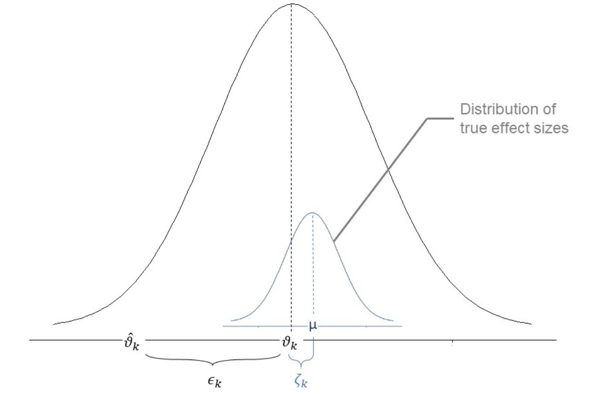
An illustration of parameters of the random-effects-model

The formula for the random-effects-model therefore looks like this:

\[\hat\theta_k = \mu + \epsilon_k + \zeta_k\]

When calculating a random-effects-model meta-analysis, where therefore also have to take the error \(\zeta_k\) into account. To do this, we have to estimate the variance of the distribution of true effect sizes, which is denoted by \(\tau^{2}\), or tau². There are several estimators for \(\tau^{2}\), all of which are implemented in metafor.

Even though it is conventional to use random-effects-model meta-analyses in psychological outcome research, applying this model is not undisputed. The random-effects-model pays more attention to small studies when pooling the overall effect in a meta-analysis (Schwarzer, Carpenter, and Rücker 2015). Yet, small studies in particular are often fraught with bias (see Chapter 8.1). This is why some have argued that the fixed-effects-model should be nearly always preferred (Poole and Greenland 1999; Furukawa, McGuire, and Barbui 2003).

5.2.1 Estimators for tau² in the random-effects-model

Operationally, conducting a random-effects-model meta-analysis in R is not so different from conducting a fixed-effects-model meta-analyis. Yet, we do have choose an estimator for \(\tau^{2}\). Here are the estimators implemented in metafor, which we can choose using the method argument when calling the function.

Code	Estimator
DL	DerSimonian-Laird
PM	Paule-Mandel
REML	Restricted Maximum-Likelihood
ML	Maximum-likelihood
HS	Hunter-Schmidt
SJ	Sidik-Jonkman
HE	Hedges
EB	Empirical Bayes

Which estimator should I use?

All of these estimators derive \(\tau^{2}\) using a slightly different approach, leading to somewhat different pooled effect size estimates and confidence intervals. If one of these approaches is more or less biased often depends on the context, and parameters such as the number of studies \(k\), the number of participants \(n\) in each study, how much \(n\) varies from study to study, and how big \(\tau^{2}\) is.

An overview paper by Veroniki and colleagues (Veroniki et al. 2016) provides an excellent summary on current evidence which estimator might be more or less biased in which situation. The article is openly accessible, and you can read it here. This paper suggests that the Restricted Maximum-Likelihood estimator performs best, and it is the default estimator in metafor.

5.2.2 Conducting the analysis

Random-effects meta-analyses are very easy to code in R. Compared to the fixed-effects-model Chapter 5.1, we can simply remove the method = "FE" argument, if we want to use the default REML estimator:

m_re <- rma(yi = df$d,     # The d-column of the df, which contains Cohen's d
            vi = df$vi)    # The vi-column of the df, which contains the variances
m_re

## 
## Random-Effects Model (k = 56; tau^2 estimator: REML)
## 
## tau^2 (estimated amount of total heterogeneity): 0.0570 (SE = 0.0176)
## tau (square root of estimated tau^2 value):      0.2388
## I^2 (total heterogeneity / total variability):   67.77%
## H^2 (total variability / sampling variability):  3.10
## 
## Test for Heterogeneity:
## Q(df = 55) = 156.9109, p-val < .0001
## 
## Model Results:
## 
## estimate      se    zval    pval   ci.lb   ci.ub 
##   0.2393  0.0414  5.7805  <.0001  0.1581  0.3204  *** 
## 
## ---
## Signif. codes:  0 '***' 0.001 '**' 0.01 '*' 0.05 '.' 0.1 ' ' 1

The output shows that our estimated effect is \(g=0.2393\), and the 95% confidence interval stretches from \(g=0.16\) to \(0.32\) (rounded). The estimated heterogeneity is \(\tau^2 = 0.06\). The percentage of variation across effect sizes that is due to heterogeneity rather than change is estimated at \(I^2 = 67.77\%\).

The summary effect estimate is different (and larger) than the one we found in the fixed-effects-model meta-analysis in Chapter 5.1 (\(g=0.21\)).

References

Borenstein, Michael, Larry V Hedges, Julian PT Higgins, and Hannah R Rothstein. 2011. Introduction to Meta-Analysis. John Wiley & Sons.

Furukawa, Toshi A, Hugh McGuire, and Corrado Barbui. 2003. “Low Dosage Tricyclic Antidepressants for Depression.” Cochrane Database of Systematic Reviews, no. 3. John Wiley & Sons, Ltd.

Poole, Charles, and Sander Greenland. 1999. “Random-Effects Meta-Analyses Are Not Always Conservative.” American Journal of Epidemiology 150 (5). Oxford University Press: 469–75.

Schwarzer, Guido, James R Carpenter, and Gerta Rücker. 2015. Meta-Analysis with R. Springer.

Veroniki, Areti Angeliki, Dan Jackson, Wolfgang Viechtbauer, Ralf Bender, Jack Bowden, Guido Knapp, Oliver Kuss, Julian PT Higgins, Dean Langan, and Georgia Salanti. 2016. “Methods to Estimate the Between-Study Variance and Its Uncertainty in Meta-Analysis.” Research Synthesis Methods 7 (1). Wiley Online Library: 55–79.