9.5 Common pitfalls
As we have mentioned before, multiple meta-regression, while very useful when applied properly, comes with certain caveats we have to know and consider when fitting a model. Indeed, some argue that (multiple) meta-regression is often improperly used and interpreted in practice, leading to a low validity of many meta-regression models (Higgins and Thompson 2004). Thus, there are some points we have to keep in mind when fitting multiple meta-regression models, which we will describe in the following.
Overfitting: seeing a signal when there is none
To better understand the risks of (multiple) meta-regression models, we have to understand the concept of overfitting. Overfitting occurs when we build a statistical model which fits the data too closely. In essence, this means that we build a statistical model which can predict the data at hand very well, but performs bad at predicting future data it has never seen before. This happens if our model assumes that some variation in our data stems from a true “signal” in our data, when in fact we only model random noise (Iniesta, Stahl, and McGuffin 2016). As a result, our statistical model produces false positive results: it sees relationships where there are none.
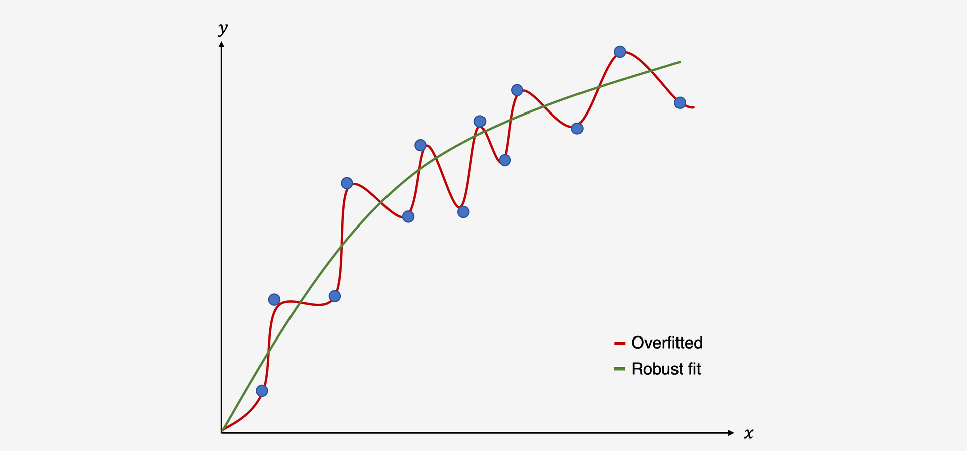
Illustration of an overfitted model vs. model with a good fit
Regression methods, which usually utilize minimization or maximization procedures such as Ordinary Least Squares or Maximum Likelihood estimatation, can be prone to overfitting (Gigerenzer 2004, 2008). Unfortunately, the risk of building a non-robust model, which produces false-positive results, is even higher once we go from conventional regression to meta-regression (Higgins and Thompson 2004). There are several reasons for this:
- In Meta-Regression, our sample of data is mostly small, as we can only use the synthesized data of all analyzed studies \(k\).
- As our meta-analysis aims to be a comprehensive overview of all evidence, we have no additional data on which we can “test” how well our regression model can predict high or low effect sizes.
- In meta-regressions, we have to deal with the potential presence of effect size heterogeneity (see Chapter 6). Imagine a case in which we have two studies with different effect sizes and non-overlapping confidence intervals. Every variable which has different values for the different studies might be a potential explanation for effect size difference we find, while it seems straightforward that most of such explanations are spurious (Higgins and Thompson 2004).
- Meta-regression as such, and multiple meta-regression in particular, make it very easy to “play around” with predictors. We can test numerous meta-regression models, include many more predictors or remove them in an attempt to explain the heterogeneity in our data. Such an approach is of course tempting, and often found in practice, because we, as meta-analysts, want to find a significant model which explains why effect sizes differ (J. Higgins et al. 2002). However, such behavior massively increases the risk of spurious findings (Higgins and Thompson 2004), because we can change parts of our model indefinitely until we find a significant model, which is then very likely to be overfitted (i.e., it mostly models statistical noise).
Some guidelines have been proposed to avoid an excessive false positive rate when building meta-regression models:
- Minimize the number of investigated predictors a priori. Predictor selection should be based on predefined scientific or theoretical questions we want to answer in our meta-regression.
- When evaluating the fit of a meta-regression model, we prefer models which achieve a good fit with less predictors. Use fit indices that balance fit and parsimony, such as the Akaike and Bayesian information criterion, to determine which model to retain if you compare several models.
-
When the number of studies is low (which is very likely to be the case), and we want to compute the significance of a predictor, you can use the Knapp-Hartung adjustment to obtain more reliable estimates (J. Higgins et al. 2002), by specifying
test = "knhawhen callingrma().
References
Gigerenzer, Gerd. 2004. “Mindless Statistics.” The Journal of Socio-Economics 33 (5). Elsevier: 587–606.
Gigerenzer, Gerd. 2008. Rationality for Mortals: How People Cope with Uncertainty. Oxford University Press.
Higgins, Julian PT, and Simon G Thompson. 2004. “Controlling the Risk of Spurious Findings from Meta-Regression.” Statistics in Medicine 23 (11). Wiley Online Library: 1663–82.
Higgins, Julian, Simon Thompson, Jonathan Deeks, and Douglas Altman. 2002. “Statistical Heterogeneity in Systematic Reviews of Clinical Trials: A Critical Appraisal of Guidelines and Practice.” Journal of Health Services Research & Policy 7 (1). SAGE Publications Sage UK: London, England: 51–61.
Iniesta, R, D Stahl, and P McGuffin. 2016. “Machine Learning, Statistical Learning and the Future of Biological Research in Psychiatry.” Psychological Medicine 46 (12). Cambridge University Press: 2455–65.