6.2 Section 1
6.2.1 Question 1.a
What is the level of measurement of each of the variables?
Click for explanation
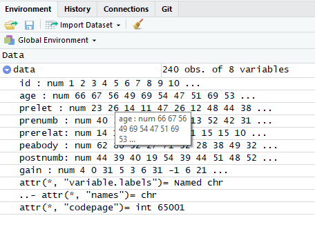
In the ‘Environment’ panel in the top right corner of the screen, click the arrow in the next to the object called ‘data.’ Alternatively, run the rode: head(data).
6.2.2 Question 1.b
What is the average age in the sample? And the range (youngest and oldest child)?
Hint: Use library(tidySEM); descriptives()
Click for explanation
As in the take home exercises, use the function descriptives() from the tidySEM package to describe the data:
library(tidySEM)
descriptives(data)
6.2.3 Question 1.c
What is the average gain in knowledge of numbers? Provide both the mean and the standard deviation.
Hint: Use the <- operator to assign to a new variable in data. You can use descriptives(), or the functions mean() and sd().
Click for explanation
Create a new variable that represents the difference between pre- and post-test scores:
data$dif <- data$postnumb - data$prenumbThere are specialized functions to obtain the mean and sd:
mean(data$dif)## [1] 9.158333sd(data$dif)## [1] 9.6824016.2.4 Question 1.d
Choose an appropriate graph to present the gain scores. What did you choose and why?
Hint: As explained in the introductory chapters, you can use ggplot and add a histogram, density plot, or boxplot: geom_histogram(); geom_density(); geom_boxplot()
Click for explanation
library(ggplot2)
p <- ggplot(data, aes(x = dif))
p + geom_histogram()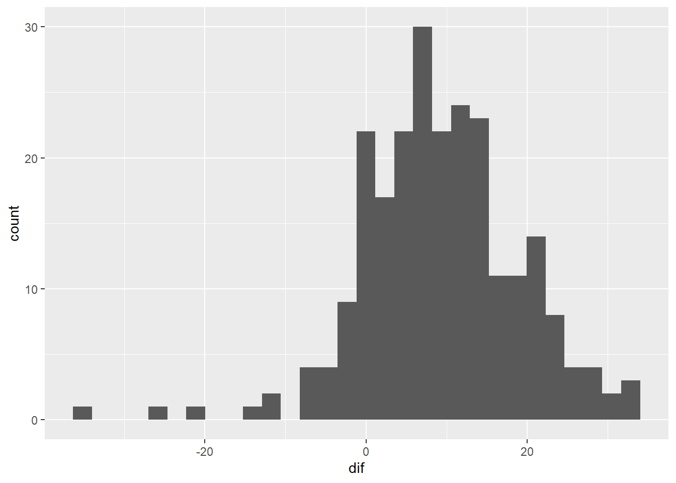
p + geom_density()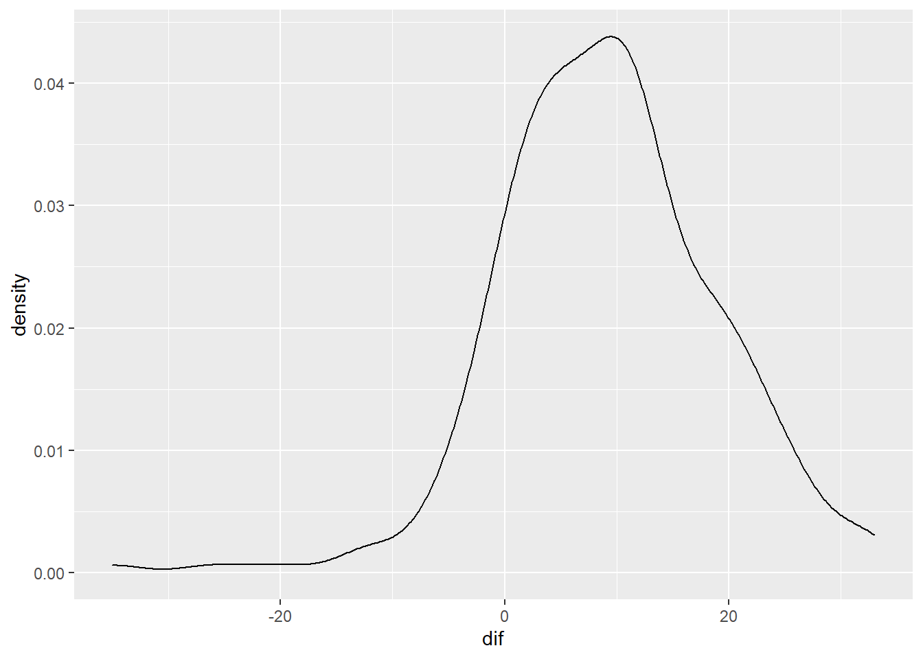
p + geom_boxplot()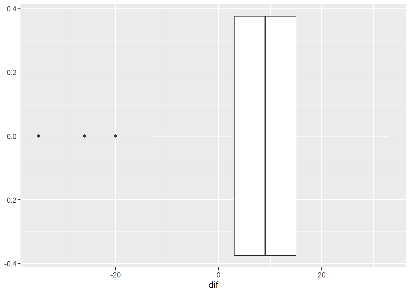
6.2.5 Question 1.e
Can you think of a graph based on two variables that is informative? What is it and how is it informative?
Hint: A useful plotting function for a bivariate distribution is the scatterplot: geom_point()
Click for explanation
#Possible variables would be the pre- and post measurement
ggplot(data, aes(x = prenumb, y = postnumb)) + geom_point()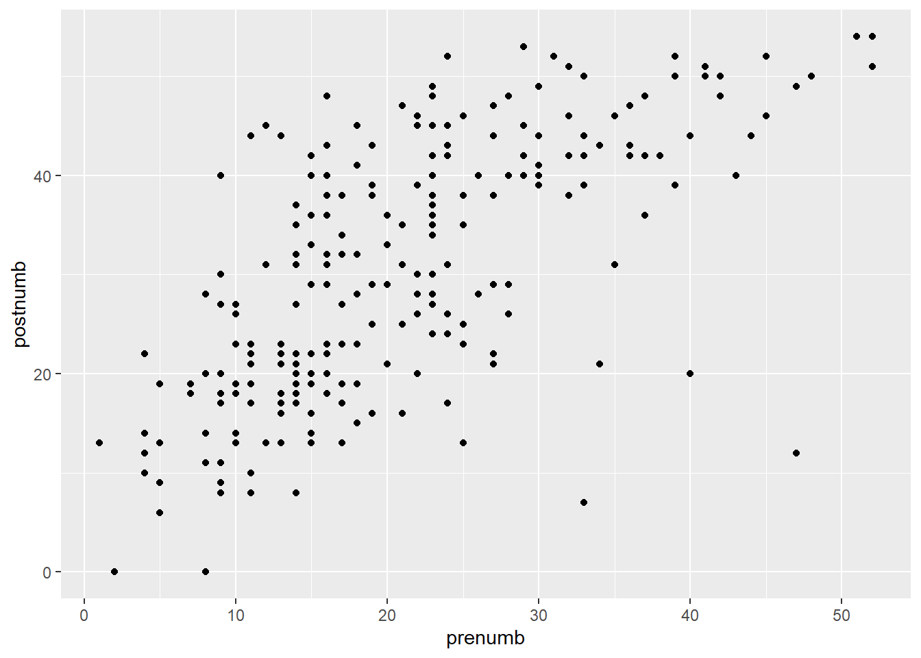
6.2.6 Question 1.f
Which of the variables age, prelet, prenumb, prerelat and peabody are related to postnumb? Use Pearson’s correlations (cor()). You don’t need to check assumptions. If you want p-values for the correlations, use the function corr.test() from the psych package instead.
Hint: The function corr.test() from the psych package provides Pearson’s correlationsand p-values (the base R function cor() does not provide p-values). Select variables by name from a data.frame object (like data) using the following syntax: data[, c("each", "variable", "name")].
Click for explanation
library(psych)
corr.test(data[, c("age", "prelet", "prenumb", "prerelat", "peabody", "postnumb")])
## Call:corr.test(x = data[, c("age", "prelet", "prenumb", "prerelat",
## "peabody", "postnumb")])
## Correlation matrix
## age prelet prenumb prerelat peabody postnumb
## age 1.00 0.33 0.43 0.44 0.29 0.34
## prelet 0.33 1.00 0.72 0.47 0.40 0.50
## prenumb 0.43 0.72 1.00 0.72 0.61 0.68
## prerelat 0.44 0.47 0.72 1.00 0.56 0.54
## peabody 0.29 0.40 0.61 0.56 1.00 0.52
## postnumb 0.34 0.50 0.68 0.54 0.52 1.00
## Sample Size
## [1] 240
## Probability values (Entries above the diagonal are adjusted for multiple tests.)
## age prelet prenumb prerelat peabody postnumb
## age 0 0 0 0 0 0
## prelet 0 0 0 0 0 0
## prenumb 0 0 0 0 0 0
## prerelat 0 0 0 0 0 0
## peabody 0 0 0 0 0 0
## postnumb 0 0 0 0 0 0
##
## To see confidence intervals of the correlations, print with the short=FALSE optionThe use of data[,] follows the conventions of matrix indexation: You can select rows (the horizontal lines) like this, data[i, ], and columns (the vertical lines) like this, data[ ,j], where i are the rows and j are the columns you want to select. As you can see in the example, you can select multiple columns using c( … , … ).
6.2.7 Question 1.g
Can age and prenumb be used to predict postnumb? If so, discuss the substantial importance of the model and the significance and substantial importance of the separate predictors.
Hint: The function lm() (short for linear model) conducts linear regression. The functions summary() provides relevant summary statistics for the model. It can be helpful to store the results of your analysis in an object, too.
Click for explanation
results <- lm(formula = postnumb ~ age + prenumb,
              data = data)
summary(results)
##
## Call:
## lm(formula = postnumb ~ age + prenumb, data = data)
##
## Residuals:
## Min 1Q Median 3Q Max
## -38.130 -6.456 -0.456 5.435 22.568
##
## Coefficients:
## Estimate Std. Error t value Pr(>|t|)
## (Intercept) 7.4242 5.1854 1.432 0.154
## age 0.1225 0.1084 1.131 0.259
## prenumb 0.7809 0.0637 12.259 <2e-16 ***
## ---
## Signif. codes: 0 '***' 0.001 '**' 0.01 '*' 0.05 '.' 0.1 ' ' 1
##
## Residual standard error: 9.486 on 237 degrees of freedom
## Multiple R-squared: 0.4592, Adjusted R-squared: 0.4547
## F-statistic: 100.6 on 2 and 237 DF, p-value: < 2.2e-166.2.8 Question 1.h
Provide the null hypotheses and the alternative hypotheses of the model in 1.g.
Click for explanation
The null-hypotheses of the model pertain to the variance explained: \(\rho^2\) (that’s Greek letter rho, for the population value of \(\rho^2\)).
\(H_0: \rho^2 = 0\)
\(H_a: \rho^2 > 0\)
6.2.9 Question 1.i
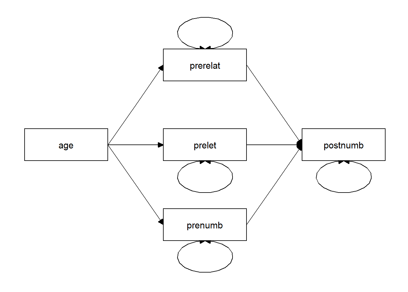
Consider the path model below. How many regression coefficients are estimated in this model? And how many variances? And how many covariances? How many degrees of freedom does this model have? (\(df = N_{obs} – N_{par}\), see slides Lecture 1).
6.2.10 Question 1.j
Consider a multiple regression analysis with three continuous independent variables, tests in language, history and logic, and one continuous dependent variable, a score on a math test. We want to know whether the various tests can predict the math score. Sketch a path model for this analysis (there are examples in the lecture slides of week 1).
How many regression parameters are there? How many variances could you estimate? How many covariances could you estimate? How many degrees of freedom does this model have?