Chapter 16 Week 3 - Class
This week, we will analyze the data from the European social survey, and the paper by Kestilä for the last time. Last week, you first replicated the results by Kestilä, and then ran your own set of factor analyses. Hopefully you experienced yourself that it matters quite a bit what type of factor analysis method you choose; both for the interpretation of your factors, and analyses that incorporate factor scores.
Instead of doing Exploratory Factor Analysis, another way of analyzing the data from the European Social Survey would be to use Confirmatory Factor Analysis. During this practical, you will conduct a CFA and compare your results to earlier EFA and PCA results and the article by Kestilä.
16.0.1 Question 1
Load the ESS data into R, into an object called df. The data are in the file "week3_class.csv". You can load it into R using the syntax:
df <- read.csv("week3_class.csv", stringsAsFactors = TRUE)Furthermore, you will have to load the package lavaan before starting with the exercises.
Click for explanation
library(lavaan)Furthermore, we want to work with numeric variables instead of factors once again, and with the countries of interest only.
Click for explanation
16.0.2 Question 2
First, review your EFA-results for the ‘trust in politics’ items, as well as the question wordings of the items. How many factors do you expect?
16.0.3 Question 3
Build a CFA model for the trust in politics items by means of the R-package lavaan. A tutorial example is available here: http://lavaan.ugent.be/tutorial/cfa.html
Make sure to ask for model fit statistics. What do you find for the value of Chi-square, df, RMSEA and CFI? Any idea why you find this Chi-square value? Does the model fit the data?
Click for explanation
trust_model_3f <- 'trustpol  =~ pltcare + pltinvt + trstplt
                   satcntry  =~ stfeco + stfgov + stfdem + stfedu + stfhlth
                   trustinst =~ trstlgl + trstplc + trstun + trstprl'

fit_trust_model_3f <- cfa(trust_model_3f, data = df)
summary(fit_trust_model_3f, fit.measures = TRUE)
## lavaan 0.6-9 ended normally after 45 iterations
##
## Estimator ML
## Optimization method NLMINB
## Number of model parameters 27
##
## Used Total
## Number of observations 15448 18187
##
## Model Test User Model:
##
## Test statistic 9188.922
## Degrees of freedom 51
## P-value (Chi-square) 0.000
##
## Model Test Baseline Model:
##
## Test statistic 75675.049
## Degrees of freedom 66
## P-value 0.000
##
## User Model versus Baseline Model:
##
## Comparative Fit Index (CFI) 0.879
## Tucker-Lewis Index (TLI) 0.844
##
## Loglikelihood and Information Criteria:
##
## Loglikelihood user model (H0) -357923.209
## Loglikelihood unrestricted model (H1) -353328.748
##
## Akaike (AIC) 715900.419
## Bayesian (BIC) 716106.840
## Sample-size adjusted Bayesian (BIC) 716021.036
##
## Root Mean Square Error of Approximation:
##
## RMSEA 0.108
## 90 Percent confidence interval - lower 0.106
## 90 Percent confidence interval - upper 0.110
## P-value RMSEA <= 0.05 0.000
##
## Standardized Root Mean Square Residual:
##
## SRMR 0.058
##
## Parameter Estimates:
##
## Standard errors Standard
## Information Expected
## Information saturated (h1) model Structured
##
## Latent Variables:
## Estimate Std.Err z-value P(>|z|)
## trustpol =~
## pltcare 1.000
## pltinvt 0.981 0.015 65.449 0.000
## trstplt 2.848 0.035 80.855 0.000
## satcntry =~
## stfeco 1.000
## stfgov 1.039 0.013 81.895 0.000
## stfdem 0.979 0.012 80.257 0.000
## stfedu 0.780 0.012 64.344 0.000
## stfhlth 0.706 0.012 58.239 0.000
## trustinst =~
## trstlgl 1.000
## trstplc 0.777 0.012 64.538 0.000
## trstun 0.861 0.013 66.949 0.000
## trstprl 1.123 0.013 85.721 0.000
##
## Covariances:
## Estimate Std.Err z-value P(>|z|)
## trustpol ~~
## satcntry 0.793 0.016 48.672 0.000
## trustinst 0.950 0.018 51.888 0.000
## satcntry ~~
## trustinst 2.046 0.040 51.736 0.000
##
## Variances:
## Estimate Std.Err z-value P(>|z|)
## .pltcare 0.651 0.008 77.811 0.000
## .pltinvt 0.680 0.009 78.658 0.000
## .trstplt 1.103 0.029 38.414 0.000
## .stfeco 2.671 0.038 70.723 0.000
## .stfgov 2.287 0.035 66.172 0.000
## .stfdem 2.266 0.033 68.444 0.000
## .stfedu 3.378 0.042 79.725 0.000
## .stfhlth 3.721 0.045 81.846 0.000
## .trstlgl 2.997 0.040 74.548 0.000
## .trstplc 3.178 0.040 80.410 0.000
## .trstun 3.443 0.043 79.405 0.000
## .trstprl 1.746 0.030 57.842 0.000
## trustpol 0.450 0.011 41.572 0.000
## satcntry 2.751 0.058 47.286 0.000
## trustinst 2.690 0.059 45.613 0.00016.0.4 Question 4
As an alternative model, build a 1-factor model, with the same items as you used before, and one trust in politics factor. Evaluate the Chi-square, df, RMSEA and CFI again. Does the one factor-model fit better or worse than the factor model you previously estimated?
Note, there is also a formal way to test whether a difference between two chi-square values is significant; more on that in the practicals of week 4.
Click for explanation
trust_model_1f <- 'political_trust =~ pltcare + pltinvt + trstprl + trstplt + stfeco + stfgov + stfdem + stfedu + stfhlth + trstlgl + trstplc + trstun + trstep'

fit_trust_model_1f <- sem(trust_model_1f, data = df)
summary(fit_trust_model_1f, fit.measures = TRUE)
## lavaan 0.6-9 ended normally after 38 iterations
##
## Estimator ML
## Optimization method NLMINB
## Number of model parameters 26
##
## Used Total
## Number of observations 14778 18187
##
## Model Test User Model:
##
## Test statistic 17667.304
## Degrees of freedom 65
## P-value (Chi-square) 0.000
##
## Model Test Baseline Model:
##
## Test statistic 81699.096
## Degrees of freedom 78
## P-value 0.000
##
## User Model versus Baseline Model:
##
## Comparative Fit Index (CFI) 0.784
## Tucker-Lewis Index (TLI) 0.741
##
## Loglikelihood and Information Criteria:
##
## Loglikelihood user model (H0) -374912.206
## Loglikelihood unrestricted model (H1) -366078.555
##
## Akaike (AIC) 749876.413
## Bayesian (BIC) 750074.036
## Sample-size adjusted Bayesian (BIC) 749991.410
##
## Root Mean Square Error of Approximation:
##
## RMSEA 0.135
## 90 Percent confidence interval - lower 0.134
## 90 Percent confidence interval - upper 0.137
## P-value RMSEA <= 0.05 0.000
##
## Standardized Root Mean Square Residual:
##
## SRMR 0.080
##
## Parameter Estimates:
##
## Standard errors Standard
## Information Expected
## Information saturated (h1) model Structured
##
## Latent Variables:
## Estimate Std.Err z-value P(>|z|)
## political_trust =~
## pltcare 1.000
## pltinvt 0.966 0.018 55.075 0.000
## trstprl 2.986 0.043 70.171 0.000
## trstplt 2.988 0.042 71.755 0.000
## stfeco 2.262 0.039 57.544 0.000
## stfgov 2.489 0.040 62.079 0.000
## stfdem 2.522 0.039 64.095 0.000
## stfedu 1.756 0.036 48.642 0.000
## stfhlth 1.554 0.035 43.930 0.000
## trstlgl 2.526 0.041 61.195 0.000
## trstplc 1.956 0.036 54.052 0.000
## trstun 2.350 0.040 59.017 0.000
## trstep 2.296 0.038 60.160 0.000
##
## Variances:
## Estimate Std.Err z-value P(>|z|)
## .pltcare 0.743 0.009 81.579 0.000
## .pltinvt 0.775 0.009 82.043 0.000
## .trstprl 1.938 0.027 70.877 0.000
## .trstplt 1.548 0.023 67.052 0.000
## .stfeco 3.565 0.044 81.289 0.000
## .stfgov 3.044 0.038 79.326 0.000
## .stfdem 2.631 0.034 78.072 0.000
## .stfedu 3.941 0.047 83.419 0.000
## .stfhlth 4.201 0.050 84.093 0.000
## .trstlgl 3.370 0.042 79.787 0.000
## .trstplc 3.410 0.041 82.311 0.000
## .trstun 3.451 0.043 80.749 0.000
## .trstep 3.019 0.038 80.272 0.000
## political_trst 0.360 0.010 36.350 0.00016.0.5 Question 5
Similarly, can you think of a 2-factor model that would explain political trust? Build this model as well, and compare Chi-square, df, RMSEA and CFI to both the 1-factor and the 3-factor model. Which of the models is the best in your opinion?
By now, you should be able to perform your own two-factor CFA, based on substantive grounds. If you do not know how to do this immediately, please have a look at question 3.
Note: None of the models fit really well. In practice, this would mean that you would have to change the model. For now, stick with the best model you have.
16.0.6 Question 6
Choose your best model, and ask for the standardized estimates by means of the addition standardized = TRUE in the summary command. Which item is the best predictor of the first factor?
Click for explanation
summary(fit_trust_model_3f, fit.measures = TRUE, standardized = TRUE)## lavaan 0.6-9 ended normally after 45 iterations
##
## Estimator ML
## Optimization method NLMINB
## Number of model parameters 27
##
## Used Total
## Number of observations 15448 18187
##
## Model Test User Model:
##
## Test statistic 9188.922
## Degrees of freedom 51
## P-value (Chi-square) 0.000
##
## Model Test Baseline Model:
##
## Test statistic 75675.049
## Degrees of freedom 66
## P-value 0.000
##
## User Model versus Baseline Model:
##
## Comparative Fit Index (CFI) 0.879
## Tucker-Lewis Index (TLI) 0.844
##
## Loglikelihood and Information Criteria:
##
## Loglikelihood user model (H0) -357923.209
## Loglikelihood unrestricted model (H1) -353328.748
##
## Akaike (AIC) 715900.419
## Bayesian (BIC) 716106.840
## Sample-size adjusted Bayesian (BIC) 716021.036
##
## Root Mean Square Error of Approximation:
##
## RMSEA 0.108
## 90 Percent confidence interval - lower 0.106
## 90 Percent confidence interval - upper 0.110
## P-value RMSEA <= 0.05 0.000
##
## Standardized Root Mean Square Residual:
##
## SRMR 0.058
##
## Parameter Estimates:
##
## Standard errors Standard
## Information Expected
## Information saturated (h1) model Structured
##
## Latent Variables:
## Estimate Std.Err z-value P(>|z|) Std.lv Std.all
## trustpol =~
## pltcare 1.000 0.671 0.639
## pltinvt 0.981 0.015 65.449 0.000 0.658 0.624
## trstplt 2.848 0.035 80.855 0.000 1.911 0.876
## satcntry =~
## stfeco 1.000 1.659 0.712
## stfgov 1.039 0.013 81.895 0.000 1.724 0.752
## stfdem 0.979 0.012 80.257 0.000 1.624 0.733
## stfedu 0.780 0.012 64.344 0.000 1.294 0.576
## stfhlth 0.706 0.012 58.239 0.000 1.171 0.519
## trustinst =~
## trstlgl 1.000 1.640 0.688
## trstplc 0.777 0.012 64.538 0.000 1.275 0.582
## trstun 0.861 0.013 66.949 0.000 1.411 0.605
## trstprl 1.123 0.013 85.721 0.000 1.842 0.812
##
## Covariances:
## Estimate Std.Err z-value P(>|z|) Std.lv Std.all
## trustpol ~~
## satcntry 0.793 0.016 48.672 0.000 0.712 0.712
## trustinst 0.950 0.018 51.888 0.000 0.863 0.863
## satcntry ~~
## trustinst 2.046 0.040 51.736 0.000 0.752 0.752
##
## Variances:
## Estimate Std.Err z-value P(>|z|) Std.lv Std.all
## .pltcare 0.651 0.008 77.811 0.000 0.651 0.591
## .pltinvt 0.680 0.009 78.658 0.000 0.680 0.611
## .trstplt 1.103 0.029 38.414 0.000 1.103 0.232
## .stfeco 2.671 0.038 70.723 0.000 2.671 0.493
## .stfgov 2.287 0.035 66.172 0.000 2.287 0.435
## .stfdem 2.266 0.033 68.444 0.000 2.266 0.462
## .stfedu 3.378 0.042 79.725 0.000 3.378 0.668
## .stfhlth 3.721 0.045 81.846 0.000 3.721 0.731
## .trstlgl 2.997 0.040 74.548 0.000 2.997 0.527
## .trstplc 3.178 0.040 80.410 0.000 3.178 0.662
## .trstun 3.443 0.043 79.405 0.000 3.443 0.633
## .trstprl 1.746 0.030 57.842 0.000 1.746 0.340
## trustpol 0.450 0.011 41.572 0.000 1.000 1.000
## satcntry 2.751 0.058 47.286 0.000 1.000 1.000
## trustinst 2.690 0.059 45.613 0.000 1.000 1.000standardizedsolution(fit_trust_model_3f)16.0.7 Question 7
Byrne (2005) states that under certain conditions, a second order CFA can be specified. Would the political trust model qualify for a second order factor model?
16.0.8 Question 8
Specify a second-order factor model and run this model. What do you conclude when you evaluate model fit? Is this model better than your model that you selected in question 6?
Click for explanation
To run a second-order factor model, you can simply add an additional line within the single quotes containing the factors that you want in the second-order factor model, like in the example below.
trust_model_3f2o <- 'trustpol  =~ pltcare + pltinvt + trstprl + trstplt
                     satcntry  =~ stfeco + stfgov + stfdem + stfedu + stfhlth
                     trustinst =~ trstlgl + trstplc + trstun + trstep
                     trust     =~ trustpol + trustinst'

fit_trust_model_3f2o <- sem(trust_model_3f2o, data = df)
summary(fit_trust_model_3f2o, fit.measures = TRUE)
## lavaan 0.6-9 ended normally after 46 iterations
##
## Estimator ML
## Optimization method NLMINB
## Number of model parameters 29
##
## Used Total
## Number of observations 14778 18187
##
## Model Test User Model:
##
## Test statistic 10116.996
## Degrees of freedom 62
## P-value (Chi-square) 0.000
##
## Model Test Baseline Model:
##
## Test statistic 81699.096
## Degrees of freedom 78
## P-value 0.000
##
## User Model versus Baseline Model:
##
## Comparative Fit Index (CFI) 0.877
## Tucker-Lewis Index (TLI) 0.845
##
## Loglikelihood and Information Criteria:
##
## Loglikelihood user model (H0) -371137.053
## Loglikelihood unrestricted model (H1) -366078.555
##
## Akaike (AIC) 742332.105
## Bayesian (BIC) 742552.531
## Sample-size adjusted Bayesian (BIC) 742460.372
##
## Root Mean Square Error of Approximation:
##
## RMSEA 0.105
## 90 Percent confidence interval - lower 0.103
## 90 Percent confidence interval - upper 0.106
## P-value RMSEA <= 0.05 0.000
##
## Standardized Root Mean Square Residual:
##
## SRMR 0.058
##
## Parameter Estimates:
##
## Standard errors Standard
## Information Expected
## Information saturated (h1) model Structured
##
## Latent Variables:
## Estimate Std.Err z-value P(>|z|)
## trustpol =~
## pltcare 1.000
## pltinvt 0.973 0.016 60.793 0.000
## trstprl 2.825 0.037 75.592 0.000
## trstplt 2.943 0.037 78.957 0.000
## satcntry =~
## stfeco 1.000
## stfgov 1.046 0.013 80.774 0.000
## stfdem 0.976 0.012 78.465 0.000
## stfedu 0.779 0.012 63.067 0.000
## stfhlth 0.705 0.012 57.172 0.000
## trustinst =~
## trstlgl 1.000
## trstplc 0.799 0.012 66.870 0.000
## trstun 0.930 0.013 72.417 0.000
## trstep 0.875 0.012 71.768 0.000
## trust =~
## trustpol 1.000
## trustinst 2.391 0.042 56.391 0.000
##
## Covariances:
## Estimate Std.Err z-value P(>|z|)
## satcntry ~~
## trust 0.797 0.016 48.523 0.000
##
## Variances:
## Estimate Std.Err z-value P(>|z|)
## .pltcare 0.687 0.009 79.196 0.000
## .pltinvt 0.718 0.009 79.838 0.000
## .trstprl 1.834 0.028 64.765 0.000
## .trstplt 1.166 0.023 50.203 0.000
## .stfeco 2.648 0.038 68.975 0.000
## .stfgov 2.255 0.035 64.065 0.000
## .stfdem 2.295 0.034 67.280 0.000
## .stfedu 3.376 0.043 77.978 0.000
## .stfhlth 3.700 0.046 80.021 0.000
## .trstlgl 2.770 0.041 67.151 0.000
## .trstplc 2.940 0.039 74.828 0.000
## .trstun 2.935 0.042 70.714 0.000
## .trstep 2.699 0.038 71.292 0.000
## .trustpol 0.035 0.004 9.165 0.000
## satcntry 2.761 0.059 46.436 0.000
## .trustinst 0.722 0.030 24.029 0.000
## trust 0.381 0.011 36.203 0.00016.0.9 Question 9
Build a new one-factor model, only using the 3 items that ask about the respondents trust in institutions with 1) trust in the legal system, 2) trust in the police and 3) trust in the UN (see below). You can also take the full model you specified in either question 6 and question 9, but you might experience that the model becomes complicated due to the large amount of arrows.
After doing this, add as predictors of the latent factor: gender, age, education in years, political interest and self-placement on the left right scale.

Estimate the model. The model doesn’t fit very well, but for now, we will stick with this model. Write down the regression coefficients (standardized and unstandardized) and relevant test statistics.
Hint: Once you add predictions to your model, you should use sem() instead of cfa().
Click for explanation
We will first have to do some recoding again. You might want to make an age variable instead of a yearborn variable, which eases the interpretation. Furthermore, a dummy for gender is more informative than just the variable gndr, although this will be treated as a dummy. You will also have to recode the variables eduyrs and lrscale to numerical variables, and you will have to make a two-category dummy for the variable polintr.
df$age <- 2002 - df$yrbrn

model_q9 <- 'trustinst =~ trstlgl + trstplc + trstun
             trustinst ~ gndr + age + eduyrs + polintr + lrscale'

fit_model_q9 <- sem(model_q9, data = df)
summary(fit_model_q9, fit.measures = TRUE, standardized = TRUE)
## lavaan 0.6-9 ended normally after 41 iterations
##
## Estimator ML
## Optimization method NLMINB
## Number of model parameters 11
##
## Used Total
## Number of observations 15524 18187
##
## Model Test User Model:
##
## Test statistic 615.470
## Degrees of freedom 10
## P-value (Chi-square) 0.000
##
## Model Test Baseline Model:
##
## Test statistic 11664.434
## Degrees of freedom 18
## P-value 0.000
##
## User Model versus Baseline Model:
##
## Comparative Fit Index (CFI) 0.948
## Tucker-Lewis Index (TLI) 0.906
##
## Loglikelihood and Information Criteria:
##
## Loglikelihood user model (H0) -99125.659
## Loglikelihood unrestricted model (H1) -98817.925
##
## Akaike (AIC) 198273.319
## Bayesian (BIC) 198357.470
## Sample-size adjusted Bayesian (BIC) 198322.513
##
## Root Mean Square Error of Approximation:
##
## RMSEA 0.062
## 90 Percent confidence interval - lower 0.058
## 90 Percent confidence interval - upper 0.067
## P-value RMSEA <= 0.05 0.000
##
## Standardized Root Mean Square Residual:
##
## SRMR 0.025
##
## Parameter Estimates:
##
## Standard errors Standard
## Information Expected
## Information saturated (h1) model Structured
##
## Latent Variables:
## Estimate Std.Err z-value P(>|z|) Std.lv Std.all
## trustinst =~
## trstlgl 1.000 1.989 0.836
## trstplc 0.802 0.014 56.879 0.000 1.596 0.731
## trstun 0.584 0.012 50.257 0.000 1.162 0.503
##
## Regressions:
## Estimate Std.Err z-value P(>|z|) Std.lv Std.all
## trustinst ~
## gndr 0.101 0.036 2.821 0.005 0.051 0.025
## age 0.000 0.001 0.084 0.933 0.000 0.001
## eduyrs 0.065 0.005 12.303 0.000 0.033 0.120
## polintr -0.147 0.023 -6.357 0.000 -0.074 -0.061
## lrscale 0.087 0.009 10.046 0.000 0.044 0.090
##
## Variances:
## Estimate Std.Err z-value P(>|z|) Std.lv Std.all
## .trstlgl 1.700 0.065 26.040 0.000 1.700 0.301
## .trstplc 2.213 0.047 46.640 0.000 2.213 0.465
## .trstun 3.996 0.050 79.266 0.000 3.996 0.747
## .trustinst 3.833 0.085 44.906 0.000 0.969 0.96916.0.10 Optional
You can plot the resulting model using semPaths():
library(semPlot)
semPaths(fit_model_q9, whatLabels = "est", rotation = 4)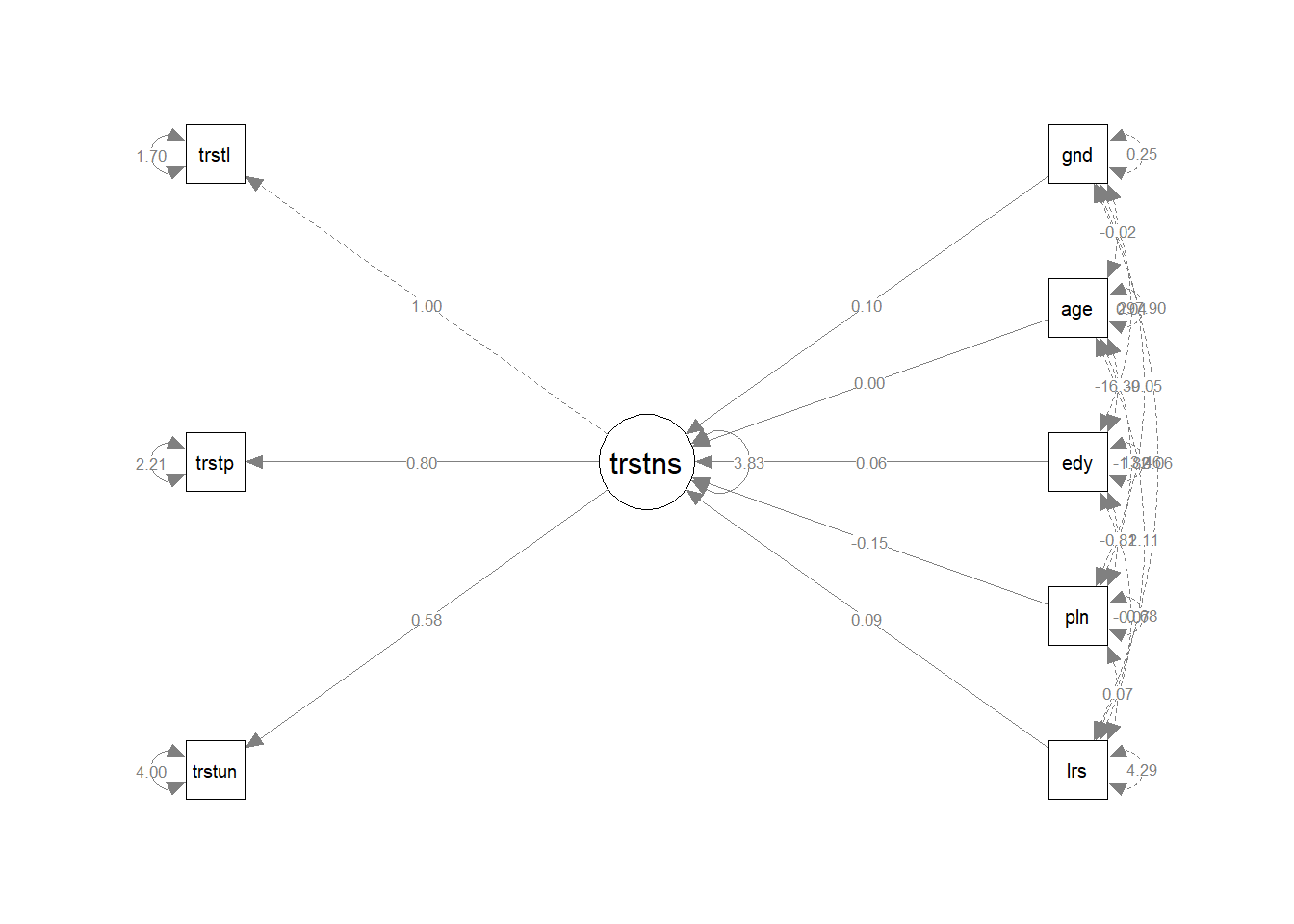
16.0.11 Question 10
Now, replace the latent score “trust in institutions” with the EFA factor score ‘trust in institutions.’ Delete the separate indicators, so you end up with the model below.

Click for explanation
model_q10 <- 'trustinstEFA ~ gndr + age + eduyrs + polintr + lrscale'

fit_model_q10 <- sem(model_q10, data = df)
summary(fit_model_q10, fit.measures = TRUE, standardized = TRUE)
## lavaan 0.6-9 ended normally after 20 iterations
##
## Estimator ML
## Optimization method NLMINB
## Number of model parameters 6
##
## Used Total
## Number of observations 13829 18187
##
## Model Test User Model:
##
## Test statistic 0.000
## Degrees of freedom 0
##
## Model Test Baseline Model:
##
## Test statistic 575.844
## Degrees of freedom 5
## P-value 0.000
##
## User Model versus Baseline Model:
##
## Comparative Fit Index (CFI) 1.000
## Tucker-Lewis Index (TLI) 1.000
##
## Loglikelihood and Information Criteria:
##
## Loglikelihood user model (H0) -19582.755
## Loglikelihood unrestricted model (H1) -19582.755
##
## Akaike (AIC) 39177.510
## Bayesian (BIC) 39222.717
## Sample-size adjusted Bayesian (BIC) 39203.649
##
## Root Mean Square Error of Approximation:
##
## RMSEA 0.000
## 90 Percent confidence interval - lower 0.000
## 90 Percent confidence interval - upper 0.000
## P-value RMSEA <= 0.05 NA
##
## Standardized Root Mean Square Residual:
##
## SRMR 0.000
##
## Parameter Estimates:
##
## Standard errors Standard
## Information Expected
## Information saturated (h1) model Structured
##
## Regressions:
## Estimate Std.Err z-value P(>|z|) Std.lv Std.all
## trustinstEFA ~
## gndr 0.146 0.017 8.537 0.000 0.146 0.072
## age -0.000 0.001 -0.443 0.658 -0.000 -0.004
## eduyrs 0.017 0.003 6.686 0.000 0.017 0.060
## polintr 0.012 0.011 1.075 0.282 0.012 0.010
## lrscale 0.087 0.004 20.970 0.000 0.087 0.176
##
## Variances:
## Estimate Std.Err z-value P(>|z|) Std.lv Std.all
## .trustinstEFA 0.994 0.012 83.153 0.000 0.994 0.959Compare the results. Does it matter whether we use a CFA or EFA to predict trust in institutions?