Chapter 25 Week 5 - Home
The data file SelfEsteem.sav contains the following variables:
- Parental Attachment
- Peer Attachment
- Empathy
- Prosocial behavior
- Aggression
- Self-esteem
Which were measured for 143 college students (mean age: 18.6 years, SD=1.61). The researcher is interested in the direct and indirect effects of parental and peer attachment on self-esteem, and the mediating roles of empathy and social behavior (i.e., prosocial behavior and aggression).
Specifically, the researcher expects that having good relationships with peers will increase prosocial behavior and decrease aggressive behavior, and that this is probably mediated through empathy (since people who experience empathy are likely to want to decrease distress in others), while the relationships with parents are expected to have a more direct effect on self-esteem.
25.0.1 Specify model
To investigate these research questions, you need to specify the model depicted below. Create a text string describing this model for later use with lavaan:
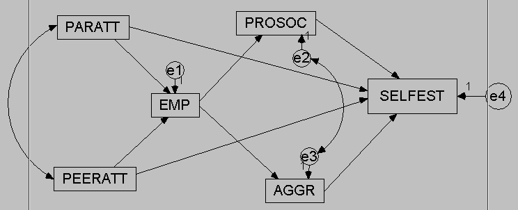
Click for explanation
mediation_model <- "SelfEst ~ ProSoc + Aggr + ParAtt + PeerAtt
                    ProSoc ~ Emp
                    Aggr ~ Emp
                    Emp ~ ParAtt + PeerAtt
                    ProSoc ~~ Aggr
                    ParAtt ~~ PeerAtt"
25.0.2 Question 1
How many and which paths are there from Parental Attachment to Self-esteem? And from Peer Attachment to Self-esteem?
Click for explanation
3 paths each; one direct, and two indirect via Emp and Prosoc/Aggr
25.0.3 Question 2
Run this model. Discuss the fit of the model.
Click for explanation
fit_mediation <- sem(mediation_model,
                     data = data)
summary(fit_mediation, fit.measures = TRUE)
## lavaan 0.6-9 ended normally after 18 iterations
##
## Estimator ML
## Optimization method NLMINB
## Number of model parameters 16
##
## Number of observations 143
##
## Model Test User Model:
##
## Test statistic 12.609
## Degrees of freedom 5
## P-value (Chi-square) 0.027
##
## Model Test Baseline Model:
##
## Test statistic 174.959
## Degrees of freedom 15
## P-value 0.000
##
## User Model versus Baseline Model:
##
## Comparative Fit Index (CFI) 0.952
## Tucker-Lewis Index (TLI) 0.857
##
## Loglikelihood and Information Criteria:
##
## Loglikelihood user model (H0) -1131.703
## Loglikelihood unrestricted model (H1) -1125.399
##
## Akaike (AIC) 2295.407
## Bayesian (BIC) 2342.812
## Sample-size adjusted Bayesian (BIC) 2292.185
##
## Root Mean Square Error of Approximation:
##
## RMSEA 0.103
## 90 Percent confidence interval - lower 0.032
## 90 Percent confidence interval - upper 0.176
## P-value RMSEA <= 0.05 0.093
##
## Standardized Root Mean Square Residual:
##
## SRMR 0.059
##
## Parameter Estimates:
##
## Standard errors Standard
## Information Expected
## Information saturated (h1) model Structured
##
## Regressions:
## Estimate Std.Err z-value P(>|z|)
## SelfEst ~
## ProSoc 0.312 0.084 3.721 0.000
## Aggr 0.159 0.083 1.915 0.056
## ParAtt 0.240 0.076 3.153 0.002
## PeerAtt 0.083 0.089 0.935 0.350
## ProSoc ~
## Emp 0.520 0.071 7.285 0.000
## Aggr ~
## Emp -0.354 0.078 -4.528 0.000
## Emp ~
## ParAtt 0.078 0.075 1.045 0.296
## PeerAtt 0.306 0.086 3.557 0.000
##
## Covariances:
## Estimate Std.Err z-value P(>|z|)
## .ProSoc ~~
## .Aggr -0.099 0.061 -1.621 0.105
## ParAtt ~~
## PeerAtt 0.537 0.103 5.215 0.000
##
## Variances:
## Estimate Std.Err z-value P(>|z|)
## .SelfEst 0.808 0.096 8.456 0.000
## .ProSoc 0.657 0.078 8.456 0.000
## .Aggr 0.789 0.093 8.456 0.000
## .Emp 0.779 0.092 8.456 0.000
## ParAtt 1.277 0.151 8.456 0.000
## PeerAtt 0.963 0.114 8.456 0.000CFI is acceptable, RMSEA is not.
25.0.4 Question 3
Considering the parameter estimates, what can you say about the research questions?
Click for explanation
The researcher expects that having good relationships with peers will increase prosocial behavior and decrease aggressive behavior, and that this is probably mediated through empathy (since people who experience empathy are likely to want to decrease distress in others), while the relationships with parents are expected to have a more direct effect on self-esteem.
Generally seems to be the case – Paratt has a significant direct effect, and ParAtt seems to have a significant effect on empathy. Need to look further at indirect effects and total effects for details.
25.0.5 Estimating indirect effects
Remember that an indirect effect is the product of several chained direct effects. Therefore, to obtain an indirect effect, you can multiply the two (or more) direct effects it consists of. Based on this knowledge - and you previous experience labelling parameters - the way to estimate indirect effects may be obvious:
- You label the direct effects
- You multiply the labels
There is a tutorial on this on the lavaan website: http://lavaan.ugent.be/tutorial/mediation.html
Additionally, a total effect is the sum of all direct and indirect effects that connect one predictor and one outcome. So, for example, in this week’s model, two indirect effects link Empathy and Self-esteem (through prosocial and aggression). The total effect of empathy on self-esteem is therefore the sum of these two indirect effects (and no direct effect).
25.0.6 Question 4
Estimate the indirect effects of Emp on SelfEst, mediated through ProSoc and Aggr. Also estimate the total effect.
Note: A new parameter is defined in lavaan using the := operator.
Click for explanation
mediation_model <- "SelfEst ~ bse_pro * ProSoc + bse_agg * Aggr + ParAtt + PeerAtt
                    ProSoc ~ bpro_emp * Emp
                    Aggr ~ bagg_emp * Emp
                    Emp ~ ParAtt + PeerAtt
                    ProSoc ~~ Aggr
                    ParAtt ~~ PeerAtt
                    ind_pro := bse_pro * bpro_emp
                    ind_agg := bse_agg * bagg_emp
                    total := ind_pro + ind_agg"
fit_mediation <- sem(mediation_model,
                     data = data)
summary(fit_mediation, fit.measures = TRUE)
## lavaan 0.6-9 ended normally after 18 iterations
##
## Estimator ML
## Optimization method NLMINB
## Number of model parameters 16
##
## Number of observations 143
##
## Model Test User Model:
##
## Test statistic 12.609
## Degrees of freedom 5
## P-value (Chi-square) 0.027
##
## Model Test Baseline Model:
##
## Test statistic 174.959
## Degrees of freedom 15
## P-value 0.000
##
## User Model versus Baseline Model:
##
## Comparative Fit Index (CFI) 0.952
## Tucker-Lewis Index (TLI) 0.857
##
## Loglikelihood and Information Criteria:
##
## Loglikelihood user model (H0) -1131.703
## Loglikelihood unrestricted model (H1) -1125.399
##
## Akaike (AIC) 2295.407
## Bayesian (BIC) 2342.812
## Sample-size adjusted Bayesian (BIC) 2292.185
##
## Root Mean Square Error of Approximation:
##
## RMSEA 0.103
## 90 Percent confidence interval - lower 0.032
## 90 Percent confidence interval - upper 0.176
## P-value RMSEA <= 0.05 0.093
##
## Standardized Root Mean Square Residual:
##
## SRMR 0.059
##
## Parameter Estimates:
##
## Standard errors Standard
## Information Expected
## Information saturated (h1) model Structured
##
## Regressions:
## Estimate Std.Err z-value P(>|z|)
## SelfEst ~
## ProSoc (bs_p) 0.312 0.084 3.721 0.000
## Aggr (bs_g) 0.159 0.083 1.915 0.056
## ParAtt 0.240 0.076 3.153 0.002
## PeerAtt 0.083 0.089 0.935 0.350
## ProSoc ~
## Emp (bpr_) 0.520 0.071 7.285 0.000
## Aggr ~
## Emp (bgg_) -0.354 0.078 -4.528 0.000
## Emp ~
## ParAtt 0.078 0.075 1.045 0.296
## PeerAtt 0.306 0.086 3.557 0.000
##
## Covariances:
## Estimate Std.Err z-value P(>|z|)
## .ProSoc ~~
## .Aggr -0.099 0.061 -1.621 0.105
## ParAtt ~~
## PeerAtt 0.537 0.103 5.215 0.000
##
## Variances:
## Estimate Std.Err z-value P(>|z|)
## .SelfEst 0.808 0.096 8.456 0.000
## .ProSoc 0.657 0.078 8.456 0.000
## .Aggr 0.789 0.093 8.456 0.000
## .Emp 0.779 0.092 8.456 0.000
## ParAtt 1.277 0.151 8.456 0.000
## PeerAtt 0.963 0.114 8.456 0.000
##
## Defined Parameters:
## Estimate Std.Err z-value P(>|z|)
## ind_pro 0.162 0.049 3.314 0.001
## ind_agg -0.056 0.032 -1.764 0.078
## total 0.106 0.051 2.066 0.03925.0.7 Question 5
Estimate all indirect effects and the total effects of Parental Attachment and Peer Attachment on Self-esteem.
Click for explanation
mediation_model <- "SelfEst ~ bse_pro * ProSoc + bse_agg * Aggr + bse_par * ParAtt + bse_peer * PeerAtt
                    ProSoc ~ bpro_emp * Emp
                    Aggr ~ bagg_emp * Emp
                    Emp ~ bemp_par * ParAtt + bemp_peer * PeerAtt
                    ProSoc ~~ Aggr
                    ParAtt ~~ PeerAtt
                    ind_par_emp_pro := bse_pro * bpro_emp * bemp_par
                    ind_peer_emp_pro := bse_pro * bpro_emp * bemp_peer
                    ind_par_emp_agg := bse_agg * bagg_emp * bemp_par
                    ind_peer_emp_agg := bse_agg * bagg_emp * bemp_peer

                    total_par := bse_par + ind_par_emp_pro + ind_par_emp_agg
                    total_peer := bse_peer + ind_peer_emp_pro + ind_peer_emp_agg"
fit_mediation <- sem(mediation_model,
                     data = data)
summary(fit_mediation)
## lavaan 0.6-9 ended normally after 18 iterations
##
## Estimator ML
## Optimization method NLMINB
## Number of model parameters 16
##
## Number of observations 143
##
## Model Test User Model:
##
## Test statistic 12.609
## Degrees of freedom 5
## P-value (Chi-square) 0.027
##
## Parameter Estimates:
##
## Standard errors Standard
## Information Expected
## Information saturated (h1) model Structured
##
## Regressions:
## Estimate Std.Err z-value P(>|z|)
## SelfEst ~
## PrS (bse_pro) 0.312 0.084 3.721 0.000
## Agg (bs_g) 0.159 0.083 1.915 0.056
## PrA (bse_par) 0.240 0.076 3.153 0.002
## PrA (bse_per) 0.083 0.089 0.935 0.350
## ProSoc ~
## Emp (bpr_) 0.520 0.071 7.285 0.000
## Aggr ~
## Emp (bgg_) -0.354 0.078 -4.528 0.000
## Emp ~
## PrA (bemp_par) 0.078 0.075 1.045 0.296
## PrA (bemp_per) 0.306 0.086 3.557 0.000
##
## Covariances:
## Estimate Std.Err z-value P(>|z|)
## .ProSoc ~~
## .Aggr -0.099 0.061 -1.621 0.105
## ParAtt ~~
## PeerAtt 0.537 0.103 5.215 0.000
##
## Variances:
## Estimate Std.Err z-value P(>|z|)
## .SelfEst 0.808 0.096 8.456 0.000
## .ProSoc 0.657 0.078 8.456 0.000
## .Aggr 0.789 0.093 8.456 0.000
## .Emp 0.779 0.092 8.456 0.000
## ParAtt 1.277 0.151 8.456 0.000
## PeerAtt 0.963 0.114 8.456 0.000
##
## Defined Parameters:
## Estimate Std.Err z-value P(>|z|)
## ind_par_emp_pr 0.013 0.013 0.997 0.319
## ind_peer_mp_pr 0.050 0.020 2.425 0.015
## ind_par_emp_gg -0.004 0.005 -0.899 0.368
## ind_peer_mp_gg -0.017 0.011 -1.580 0.114
## total_par 0.248 0.076 3.247 0.001
## total_peer 0.115 0.088 1.305 0.19225.0.8 Question 6
To compare the total effect of parental attachment versus peer attachment on self esteem, should you use the standardized or unstandardized parameters? Obtain the appropriate output, and draw a conclusion.
Click for explanation
You should use the standardized results:
summary(fit_mediation, fit.measures = TRUE, standardize = TRUE)## lavaan 0.6-9 ended normally after 18 iterations
##
## Estimator ML
## Optimization method NLMINB
## Number of model parameters 16
##
## Number of observations 143
##
## Model Test User Model:
##
## Test statistic 12.609
## Degrees of freedom 5
## P-value (Chi-square) 0.027
##
## Model Test Baseline Model:
##
## Test statistic 174.959
## Degrees of freedom 15
## P-value 0.000
##
## User Model versus Baseline Model:
##
## Comparative Fit Index (CFI) 0.952
## Tucker-Lewis Index (TLI) 0.857
##
## Loglikelihood and Information Criteria:
##
## Loglikelihood user model (H0) -1131.703
## Loglikelihood unrestricted model (H1) -1125.399
##
## Akaike (AIC) 2295.407
## Bayesian (BIC) 2342.812
## Sample-size adjusted Bayesian (BIC) 2292.185
##
## Root Mean Square Error of Approximation:
##
## RMSEA 0.103
## 90 Percent confidence interval - lower 0.032
## 90 Percent confidence interval - upper 0.176
## P-value RMSEA <= 0.05 0.093
##
## Standardized Root Mean Square Residual:
##
## SRMR 0.059
##
## Parameter Estimates:
##
## Standard errors Standard
## Information Expected
## Information saturated (h1) model Structured
##
## Regressions:
## Estimate Std.Err z-value P(>|z|) Std.lv Std.all
## SelfEst ~
## PrS (bse_pro) 0.312 0.084 3.721 0.000 0.312 0.295
## Agg (bs_g) 0.159 0.083 1.915 0.056 0.159 0.150
## PrA (bse_par) 0.240 0.076 3.153 0.002 0.240 0.269
## PrA (bse_per) 0.083 0.089 0.935 0.350 0.083 0.081
## ProSoc ~
## Emp (bpr_) 0.520 0.071 7.285 0.000 0.520 0.520
## Aggr ~
## Emp (bgg_) -0.354 0.078 -4.528 0.000 -0.354 -0.354
## Emp ~
## PrA (bemp_par) 0.078 0.075 1.045 0.296 0.078 0.093
## PrA (bemp_per) 0.306 0.086 3.557 0.000 0.306 0.316
##
## Covariances:
## Estimate Std.Err z-value P(>|z|) Std.lv Std.all
## .ProSoc ~~
## .Aggr -0.099 0.061 -1.621 0.105 -0.099 -0.137
## ParAtt ~~
## PeerAtt 0.537 0.103 5.215 0.000 0.537 0.485
##
## Variances:
## Estimate Std.Err z-value P(>|z|) Std.lv Std.all
## .SelfEst 0.808 0.096 8.456 0.000 0.808 0.797
## .ProSoc 0.657 0.078 8.456 0.000 0.657 0.729
## .Aggr 0.789 0.093 8.456 0.000 0.789 0.875
## .Emp 0.779 0.092 8.456 0.000 0.779 0.863
## ParAtt 1.277 0.151 8.456 0.000 1.277 1.000
## PeerAtt 0.963 0.114 8.456 0.000 0.963 1.000
##
## Defined Parameters:
## Estimate Std.Err z-value P(>|z|) Std.lv Std.all
## ind_par_emp_pr 0.013 0.013 0.997 0.319 0.013 0.014
## ind_peer_mp_pr 0.050 0.020 2.425 0.015 0.050 0.048
## ind_par_emp_gg -0.004 0.005 -0.899 0.368 -0.004 -0.005
## ind_peer_mp_gg -0.017 0.011 -1.580 0.114 -0.017 -0.017
## total_par 0.248 0.076 3.247 0.001 0.248 0.279
## total_peer 0.115 0.088 1.305 0.192 0.115 0.11225.0.9 Difference between parameters
To test the difference between parameters, you can constrain them to be equal and do a chi-square difference test to compare the constrained and unconstrained models. However, you can also calculate the difference between parameters, and test if it’s significant:
"dif_par_peer := total_par - total_peer"25.0.10 Bootstrapping
You may have learned before that the sampling distribution of indirect effects is not normal. Consequently, you cannot use parameteric p-values to determine the significance of indirect effects because they are biased. If you want to know whether the indirect effects are significant, you can bootstrap them to obtain a 95% confidence interval.
Bootstrapping means that lavaan will draw 1000 samples from the data and estimate the model on each sample. There will thus be 1000 estimates for every parameter. The lower and upper bounds of a 95% confidence interval are determined by taking the 2.5% and 97.5% quantiles of the 1000 samples for each parameter.
The confidence interval is interpreted the same as a normal confidence interval: If zero lies inside the interval (e.g., lower bound is -.4 and upper bound is .9), we conclude that the parameter is not significantly different from zero, but if zero does not lie in this interval (e.g., lower bound is .4 and upper bound is 1.3), we can say the parameter differs from zero (at an alpha of .05 since we are considering a 95% confidence interval).
We will get these intervals for all the parameters in the model, but we are specifically interested in the intervals for the indirect effects, because we want to know if they differ from zero (i.e., whether there is a mediated effect).
In lavaan, bootstrap standard errors are requested by specifying se = “bootstrap” in the fitting function, and specifying the number of bootstrap samples as bootstrap = 1000. First, just get your code running by specifying a low number, like 100 or even 10. Note: To draw reliable conclusions from the results, you should always use 1000+ bootstrap samples - but it can take a long time.
fit_mediation <- sem(mediation_model,
                     data = data,
                     se = "bootstrap",
                     bootstrap = 100)
To obtain the confidence intervals for your model, use the following syntax:
parameterestimates(fit_mediation, boot.ci.type = "bca.simple", standardized = TRUE)25.0.11 Question 7
What do you conclude about the indirect and total effects of Parental attachment and Peer attachment on Self-esteem? Report your conclusions as you would report them in a paper (in words and statistics).