Chapter 15 Week 3 - Home
Last week, you have worked on the data used by Kestilä in a paper that discussed two possible reasons why there is no Radical Right party in Finland. You have attempted to 1) replicate her study by doing a Principal Component Analysis and 2) a factor analysis (exploratory) of the same data.
This week you also learned that it is possible to do Confirmatory Factor Analysis within the structural
equation modeling (SEM) framework. We use the R-package lavaan to fit these kinds of models.
Before we will analyze the Kestilä data, you first need to learn some of the basic principles of doing
analyses using lavaan. Using syntax, you need to tell lavaan exactly
what kind of model you want it to estimate This opens up many more possibilities to do Theory Construction and then
subsequently test your theory using Statistical Modeling.
As a preparation for the next practical, work your way through this tutorial (part of which consists of the official lavaan tutorial). You will find that lavaan is a very user-friendly software package.
15.0.1 Get started with lavaan
To get started with lavaan, read and run the following two chapters of the official lavaan tutorial:
- Installing lavaan
- Lavaan syntax (you just have to read this one)
15.0.2 Regression models in lavaan
Download the data file Hamilton.csv, or Hamilton.xls here. The data are as follows:
Hamilton (1990) provided several measurements on each of 21 states. Three of the measurements will be used in this tutorial:
- Average SAT score
- Per capita income expressed in $1,000 units
- Median education for residents 25 years of age or older
Load the data from the .csv or .xls file into R.
Hint: Use read.csv() or readxl::read_excel()
Click for explanation
library(readxl)
df <- read_excel("Hamilton.xlsx", 1)
Or
df <- read.csv("Hamilton.csv")15.0.3 Conceptual model
The following path diagram shows a model for these data:
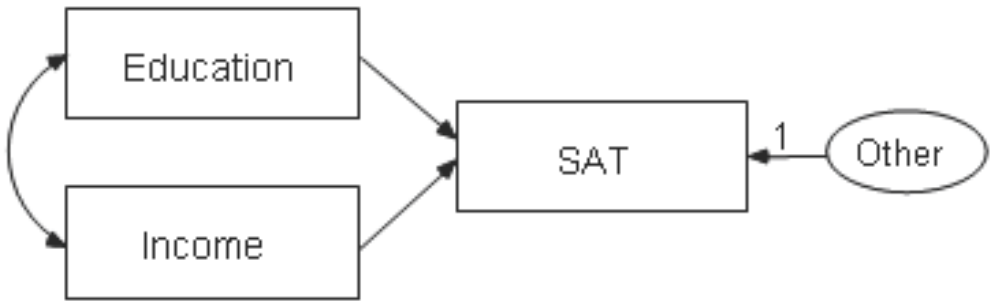
This is a simple regression model where one observed variable, SAT, is predicted as a
linear combination of the other two observed variables, Education and Income. As with
nearly all empirical data, the prediction will not be perfect. The variable Other
represents variables other than Education and Income that affect SAT.
Each single-headed arrow represents a regression weight. The number 1 in the
figure specifies that Other must have a weight of 1 in the prediction of SAT. This constraint is imposed by default in lavaan.
15.0.4 Lavaan syntax
Based on the lavaan tutorial, write down (just as text) the model syntax that describes the model in the picture. How many regressions are there? How many covariances?
Click for explanation
The syntax for this model is:
"SAT ~ Income + Education
Income ~~ Education"
Or, equivalently:
"SAT ~ Income
SAT ~ Education
Income ~~ Education"
This syntax specifies two regression equations and one covariance. However, three more parameters are included by lavaan per default:
- The residual (unexplained) variance in SAT
- The variance of Income
- The variance of Education
So, strictly speaking, if you don’t want to rely on the default settings, the syntax would be:
"SAT ~ Income + Education
Income ~~ Education
SAT~~SAT
Income~~Income
Education~~Education"
15.0.5 Performing the analysis
In lavaan, models are fit using the sem() function. Run the command ?sem to open the help file for this function. Try to figure out how to take the syntax you wrote for the previous question, and fit it to the Hamilton data.
Click for explanation
# Load the lavaan package
library(lavaan)
# Fit the model to df, and store the result in an object called 'fit'
fit <- sem(model = "SAT ~ Income + Education
                    Income ~~ Education",
           data = df)
This will result in a warning about the variances. You can ignore this.
15.0.6 Viewing the output
Most of the relevant output of a lavaan analysis can be extracted using the summary() function. Get a summary for the analysis now. Do either of the predictors have a significant effect on SA? By specifying the option rsquare = TRUE in the summary() function, you can additionally get squared multiple correlations for the dependent variables.
Click for explanation
summary(fit, rsquare = TRUE)## lavaan 0.6-9 ended normally after 48 iterations
##
## Estimator ML
## Optimization method NLMINB
## Number of model parameters 6
##
## Number of observations 21
##
## Model Test User Model:
##
## Test statistic 0.000
## Degrees of freedom 0
##
## Parameter Estimates:
##
## Standard errors Standard
## Information Expected
## Information saturated (h1) model Structured
##
## Regressions:
## Estimate Std.Err z-value P(>|z|)
## SAT ~
## Income 2.156 3.050 0.707 0.480
## Education 136.022 29.819 4.562 0.000
##
## Covariances:
## Estimate Std.Err z-value P(>|z|)
## Income ~~
## Education 0.127 0.064 2.000 0.046
##
## Variances:
## Estimate Std.Err z-value P(>|z|)
## .SAT 382.736 118.115 3.240 0.001
## Income 2.562 0.791 3.240 0.001
## Education 0.027 0.008 3.240 0.001
##
## R-Square:
## Estimate
## SAT 0.60315.0.7 Plotting the output
The package semPlot can automatically plot simple SEM models, like path models and CFA models. To visualize this SEM model, install the semPlot package, and use the function semPaths:
install.packages("semPlot")
library(semPlot)
semPaths(fit)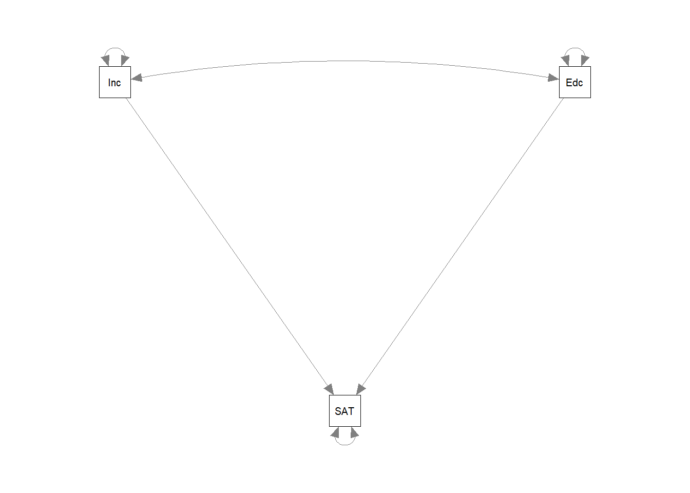
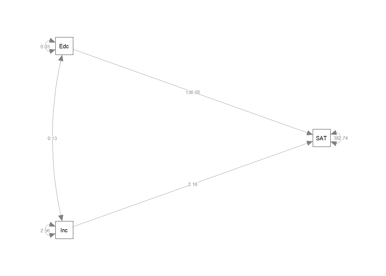
The default plot can be improved upon, for example, by plotting the parameter estimates onto the paths, and rotating it to match our initial conceptual model at the start of this tutorial:
semPaths(fit, whatLabels = "est", rotation = 2)