Chapter 20 Week 4 - Home
Load the data file SocialRejection.sav into R. It contains three variables: Condition (IV), SelfEst (IV), and Spent (DV).
20.0.1 Question 1
Check the assumption of homogeneous regression lines (no interaction) first. What is your conclusion?
Hint: You need to estimate a model with, and one without an interaction, and compare them using the anova() function.
Click for explanation
ancova_main <- aov(Spent ~ Condition + SelfEst, data = data)
ancova_int <- aov(Spent ~ Condition*SelfEst, data = data)
anova(ancova_main, ancova_int)
The lines are homogeneous, the assumption is met (interaction is not significant).
20.0.2 Question 2
What should you do when this assumption is violated?
20.0.3 Question 3
Before you can do an ANCOVA, you should also check the assumption of homogeneity. What does homogeneity imply, and is the assumption met?
Hint: You did this in the Week 1 class exercise.
Click for explanation
We can do a test of homogeneity of the variances of Spent across conditions:
bartlett.test(formula = Spent~Condition, data = data)##
## Bartlett test of homogeneity of variances
##
## data: Spent by Condition
## Bartlett's K-squared = 0.16678, df = 2, p-value = 0.92However, note that the assumption of homogeneity actually requires the residual variance, after controlling for the covariate SelfEst, to be the same across conditions. We can extract these residuals from a regression with only SelfEst as a predictor:
reg_selfest <- lm(Spent ~ SelfEst, data = data)
residuals_selfest <- reg_selfest$residuals
Then, we can test the null hypothesis that the error variance of the dependent variable is equal across groups:
bartlett.test(residuals_selfest, data$Condition)##
## Bartlett test of homogeneity of variances
##
## data: residuals_selfest and data$Condition
## Bartlett's K-squared = 0.92603, df = 2, p-value = 0.6294The test is not significant, meaning that the error variances are indeed equal, the assumption is met.
20.0.4 Question 4
What should you do when this assumption is violated?
Click for explanation
You cannot really “solve” this problem in classical regression or ANCOVA, because only one parameter is estimated for the error variance. In SEM, however, you can estimate different error variance parameters for each group.
20.0.5 Question 5
Run the actual ANCOVA (or use previous output). What are your conclusions about the effects of the factor and the covariate?
Click for explanation
summary(ancova_main)## Df Sum Sq Mean Sq F value Pr(>F)
## Condition 2 126.8 63.4 4.402 0.0169 *
## SelfEst 1 419.5 419.5 29.118 1.49e-06 ***
## Residuals 55 792.4 14.4
## ---
## Signif. codes: 0 '***' 0.001 '**' 0.01 '*' 0.05 '.' 0.1 ' ' 1Self esteem is significant, F (1, 55) = 29.118, p < .001, the level of self esteem of the respondent is related to the amount spent. Condition is significant after controlling for the effect of self-esteem, F (2, 55) = 4.402, p = .017, the amount spent differs between the three conditions.
20.0.6 Question 6
Let’s examine the differences in conditional means between the three conditions. In order to do so, we can use several approaches.
20.0.6.1 Approach 1: Conditional means
We can obtain the conditional means of the three groups by asking for the predicted (expected) value, based on the model, for each of the three conditions, keeping the covariate constant at 0. For this, we apply the predict() function to the object containing our analysis. We make a small new dataset for the values that we want predictions for:
new_data <- data.frame(Condition = c("rejection", "neutral", "confirming"),
                       SelfEst = c(0, 0, 0))
predict(ancova_main, new_data)
## 1 2 3
## 12.449100 10.265532 9.152918What are your conclusions about the three conditions (i.e., how do they differ)?
20.0.6.2 Approach 2: Testing significance
We can test the significance for these differences using TukeyHSD() again, but to get the conditional means, we need to use the residuals from a model that includes only SelfEst, which we obtained before:
reg_selfest <- lm(Spent ~ SelfEst, data = data)
residuals_selfest <- reg_selfest$residuals
anova_conditional <- aov(residuals_selfest ~ data$Condition)
TukeyHSD(anova_conditional)
## Tukey multiple comparisons of means
## 95% family-wise confidence level
##
## Fit: aov(formula = residuals_selfest ~ data$Condition)
##
## $`data$Condition`
## diff lwr upr p adj
## neutral-rejection -2.174775 -5.076198 0.7266467 0.1773921
## confirming-rejection -3.296276 -6.197698 -0.3948536 0.0223500
## confirming-neutral -1.121500 -3.985483 1.7424826 0.6157693Respondents in the rejection condition spent more, than respondents in the neutral condition and the confirming condition. These differences are not tested on significance between two groups.
20.0.6.3 Approach 3: Plotting the difference
This is where R really shines: We can quickly put together a plot that shows the difference between groups, along with the raw data. We use the package ggplot2
library(ggplot2)
# Put the data for the plot together
plot_data <- data.frame(Spent_resid = residuals_selfest,
                        Condition = data$Condition)
# Basic plot; indicate that you want condition on the x-axis and Spent_resid on
# the y-axis
ggplot(plot_data, aes(x = Condition, y = Spent_resid)) +
  geom_boxplot() + # Add a boxplot for each condition
  geom_jitter(width = .2) + # Plot raw datapoints on top
  theme_bw() # Add a nice APA theme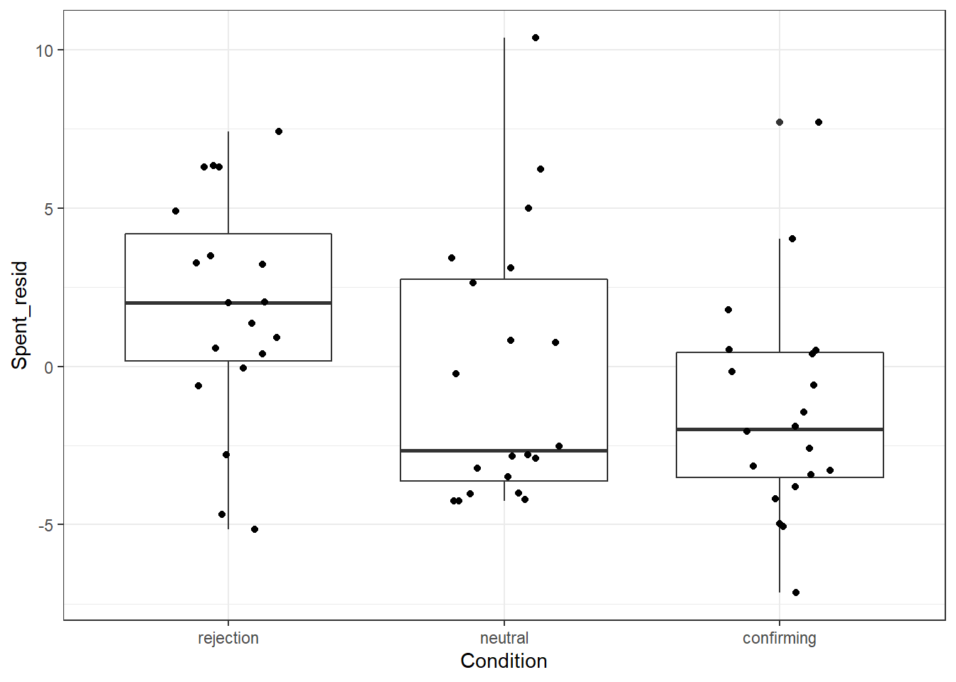
20.0.7 Question 7
An AN(C)OVA can also be specified as a regression analysis. R automatically creates dummies. Use the lm() function instead of aov(), and compare the results.
Click for explanation
ancova_main <- aov(Spent ~ Condition + SelfEst, data = data)
summary(ancova_main)
## Df Sum Sq Mean Sq F value Pr(>F)
## Condition 2 126.8 63.4 4.402 0.0169 *
## SelfEst 1 419.5 419.5 29.118 1.49e-06 ***
## Residuals 55 792.4 14.4
## ---
## Signif. codes: 0 '***' 0.001 '**' 0.01 '*' 0.05 '.' 0.1 ' ' 1lm_main <- lm(Spent ~ Condition + SelfEst, data = data)
summary(lm_main)##
## Call:
## lm(formula = Spent ~ Condition + SelfEst, data = data)
##
## Residuals:
## Min 1Q Median 3Q Max
## -6.9987 -2.5886 -0.4841 1.9772 10.6503
##
## Coefficients:
## Estimate Std. Error t value Pr(>|t|)
## (Intercept) 12.44910 1.98050 6.286 5.54e-08 ***
## Conditionneutral -2.18357 1.22451 -1.783 0.08007 .
## Conditionconfirming -3.29618 1.21599 -2.711 0.00894 **
## SelfEst -0.52406 0.09712 -5.396 1.49e-06 ***
## ---
## Signif. codes: 0 '***' 0.001 '**' 0.01 '*' 0.05 '.' 0.1 ' ' 1
##
## Residual standard error: 3.796 on 55 degrees of freedom
## Multiple R-squared: 0.4081, Adjusted R-squared: 0.3758
## F-statistic: 12.64 on 3 and 55 DF, p-value: 2.142e-06You can get the conditional means directly from this lm() model by dropping the intercept, using -1 (which means: minus the intercept) in the formula:
lm_no_intercept <- lm(Spent ~ -1 + Condition + SelfEst, data = data)
summary(lm_no_intercept)
##
## Call:
## lm(formula = Spent ~ -1 + Condition + SelfEst, data = data)
##
## Residuals:
## Min 1Q Median 3Q Max
## -6.9987 -2.5886 -0.4841 1.9772 10.6503
##
## Coefficients:
## Estimate Std. Error t value Pr(>|t|)
## Conditionrejection 12.44910 1.98050 6.286 5.54e-08 ***
## Conditionneutral 10.26553 2.10191 4.884 9.35e-06 ***
## Conditionconfirming 9.15292 1.96952 4.647 2.14e-05 ***
## SelfEst -0.52406 0.09712 -5.396 1.49e-06 ***
## ---
## Signif. codes: 0 '***' 0.001 '**' 0.01 '*' 0.05 '.' 0.1 ' ' 1
##
## Residual standard error: 3.796 on 55 degrees of freedom
## Multiple R-squared: 0.4218, Adjusted R-squared: 0.3797
## F-statistic: 10.03 on 4 and 55 DF, p-value: 3.616e-0620.0.8 Question 8
To perform this analysis as a structural equation model, we need to manually compute dummy variables. We can use the function model.matrix() to “expand” a factor variable into dummies:
data_dummies <- model.matrix(~ -1 + Condition, data = data)
head(data_dummies)
## Conditionrejection Conditionneutral Conditionconfirming
## 1 1 0 0
## 2 1 0 0
## 3 1 0 0
## 4 1 0 0
## 5 1 0 0
## 6 1 0 0We can then bind these columns with dummies to our original data using cbind() (column bind):
data <- cbind(data, data_dummies)
head(data)
Begin by specifying the model in lavaan like this:

Click for explanation
library(lavaan)
ancova_lavaan <- sem('Spent ~ SelfEst + Conditionrejection + Conditionconfirming', data = data)
summary(ancova_lavaan)
## lavaan 0.6-9 ended normally after 21 iterations
##
## Estimator ML
## Optimization method NLMINB
## Number of model parameters 4
##
## Number of observations 59
##
## Model Test User Model:
##
## Test statistic 0.000
## Degrees of freedom 0
##
## Parameter Estimates:
##
## Standard errors Standard
## Information Expected
## Information saturated (h1) model Structured
##
## Regressions:
## Estimate Std.Err z-value P(>|z|)
## Spent ~
## SelfEst -0.524 0.094 -5.589 0.000
## Conditionrjctn 2.184 1.182 1.847 0.065
## Conditncnfrmng -1.113 1.167 -0.953 0.341
##
## Variances:
## Estimate Std.Err z-value P(>|z|)
## .Spent 13.430 2.473 5.431 0.000To obtain a plot of these results and compare it to our picture above, use SemPlot:
library(semPlot)
semPaths(ancova_lavaan, whatLabels = "est", rotation = 2)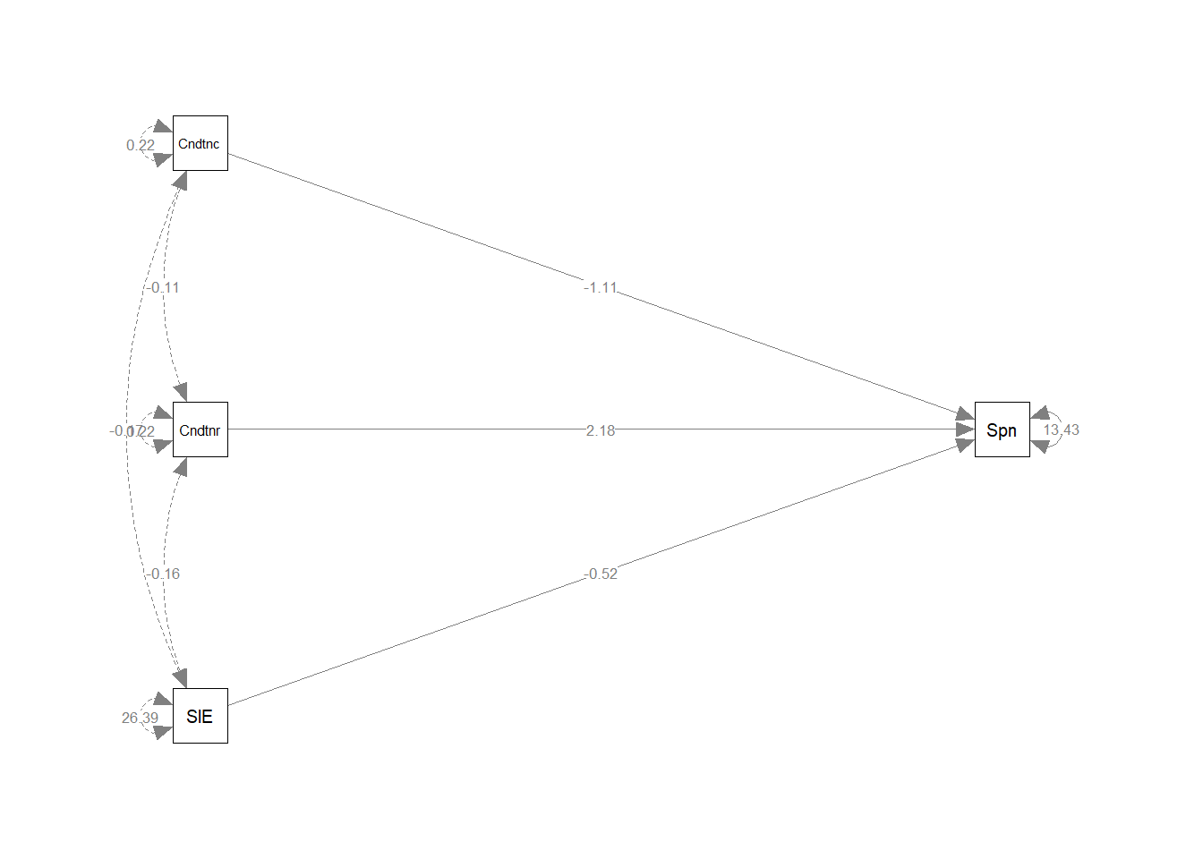
20.0.9 Additional options
Note: When you are doing an ANCOVA (even as a regression model with dummies), you want to analyze both the covariance structure AND the mean structure. To include the latter in your analysis, you have to tell lavaan to include this by adding the argument meanstructure = TRUE in the fitting function:
library(lavaan)
ancova_lavaan <- sem('Spent ~ SelfEst + Conditionrejection + Conditionconfirming',
                     data = data,
                     meanstructure = TRUE)
summary(ancova_lavaan)
## lavaan 0.6-9 ended normally after 35 iterations
##
## Estimator ML
## Optimization method NLMINB
## Number of model parameters 5
##
## Number of observations 59
##
## Model Test User Model:
##
## Test statistic 0.000
## Degrees of freedom 0
##
## Parameter Estimates:
##
## Standard errors Standard
## Information Expected
## Information saturated (h1) model Structured
##
## Regressions:
## Estimate Std.Err z-value P(>|z|)
## Spent ~
## SelfEst -0.524 0.094 -5.589 0.000
## Conditionrjctn 2.184 1.182 1.847 0.065
## Conditncnfrmng -1.113 1.167 -0.953 0.341
##
## Intercepts:
## Estimate Std.Err z-value P(>|z|)
## .Spent 10.266 2.029 5.058 0.000
##
## Variances:
## Estimate Std.Err z-value P(>|z|)
## .Spent 13.430 2.473 5.431 0.000To obtain the standardized results and the proportion of explained variance (= squared multiple correlation, i.e., R2), you can use the options in the summary() function:
summary(ancova_lavaan, standardized = TRUE, rsquare = TRUE)## lavaan 0.6-9 ended normally after 35 iterations
##
## Estimator ML
## Optimization method NLMINB
## Number of model parameters 5
##
## Number of observations 59
##
## Model Test User Model:
##
## Test statistic 0.000
## Degrees of freedom 0
##
## Parameter Estimates:
##
## Standard errors Standard
## Information Expected
## Information saturated (h1) model Structured
##
## Regressions:
## Estimate Std.Err z-value P(>|z|) Std.lv Std.all
## Spent ~
## SelfEst -0.524 0.094 -5.589 0.000 -0.524 -0.565
## Conditionrjctn 2.184 1.182 1.847 0.065 2.184 0.214
## Conditncnfrmng -1.113 1.167 -0.953 0.341 -1.113 -0.111
##
## Intercepts:
## Estimate Std.Err z-value P(>|z|) Std.lv Std.all
## .Spent 10.266 2.029 5.058 0.000 10.266 2.155
##
## Variances:
## Estimate Std.Err z-value P(>|z|) Std.lv Std.all
## .Spent 13.430 2.473 5.431 0.000 13.430 0.592
##
## R-Square:
## Estimate
## Spent 0.40820.0.10 Question 9
Compare your results to those obtained with the regression analysis. What is your conclusion?
20.0.11 Question 10
Check the model fit. What do you conclude?
Note: Use summary() and fit.measures = TRUE
Click for explanation
summary(ancova_lavaan, fit.measures = TRUE)## lavaan 0.6-9 ended normally after 35 iterations
##
## Estimator ML
## Optimization method NLMINB
## Number of model parameters 5
##
## Number of observations 59
##
## Model Test User Model:
##
## Test statistic 0.000
## Degrees of freedom 0
##
## Model Test Baseline Model:
##
## Test statistic 30.941
## Degrees of freedom 3
## P-value 0.000
##
## User Model versus Baseline Model:
##
## Comparative Fit Index (CFI) 1.000
## Tucker-Lewis Index (TLI) 1.000
##
## Loglikelihood and Information Criteria:
##
## Loglikelihood user model (H0) -160.344
## Loglikelihood unrestricted model (H1) -160.344
##
## Akaike (AIC) 330.689
## Bayesian (BIC) 341.077
## Sample-size adjusted Bayesian (BIC) 325.353
##
## Root Mean Square Error of Approximation:
##
## RMSEA 0.000
## 90 Percent confidence interval - lower 0.000
## 90 Percent confidence interval - upper 0.000
## P-value RMSEA <= 0.05 NA
##
## Standardized Root Mean Square Residual:
##
## SRMR 0.000
##
## Parameter Estimates:
##
## Standard errors Standard
## Information Expected
## Information saturated (h1) model Structured
##
## Regressions:
## Estimate Std.Err z-value P(>|z|)
## Spent ~
## SelfEst -0.524 0.094 -5.589 0.000
## Conditionrjctn 2.184 1.182 1.847 0.065
## Conditncnfrmng -1.113 1.167 -0.953 0.341
##
## Intercepts:
## Estimate Std.Err z-value P(>|z|)
## .Spent 10.266 2.029 5.058 0.000
##
## Variances:
## Estimate Std.Err z-value P(>|z|)
## .Spent 13.430 2.473 5.431 0.000Saturated model, so perfect fit. Because the number of parameters to be estimated is equal to the number of observed statistics, there is a perfect fit. Here our interest is mainly in getting the estimates, not in the model-fit.