Chapter 10 Week 2 - Home

This exercise is based on:

Kestilä, Elina (2006). Is There Demand for Radical Right Populism in the Finnish Electorate? Scandinavian Political Studies 29(3),169-191

You have read and answered questions about the article in the reading questions. In this exercise, as well as in the second class practical, we will analyze these data ourselves.

The data for this practical stem from the first round of the European Social Survey (ESS). This is a repeated cross-sectional survey across 32 European countries. The first round was held in 2002, and since then, subsequent rounds of data-collection are held bi- anually. More info, as well as access to all data -> www.europeansocialsurvey.org.

The raw, first round data can also be found here. The file is called ESSround1- a.sav. This file contains data for all respondents, but only those variables are included that you will need in this exercise.

10.0.1 Question 1.a

Download the file, and import it in R. Inspect the file (no. of cases and no. of variables) to see if the file opened well.

For a description of all variables in the dataset, click here!

Variable	Description
name	Title of dataset
essround	ESS round
edition	Edition
proddate	Production date
cntry	Country
idno	Respondent’s identification number
trstlgl	Trust in the legal system
trstplc	Trust in the police
trstun	Trust in the United Nations
trstep	Trust in the European Parliament
trstprl	Trust in country’s parliament
stfhlth	State of health services in country nowadays
stfedu	State of education in country nowadays
stfeco	How satisfied with present state of economy in country
stfgov	How satisfied with the national government
stfdem	How satisfied with the way democracy works in country
pltinvt	Politicians interested in votes rather than peoples opinions
pltcare	Politicians in general care what people like respondent think
trstplt	Trust in politicians
imsmetn	Allow many/few immigrants of same race/ethnic group as majority
imdfetn	Allow many/few immigrants of different race/ethnic group from majority
eimrcnt	Allow many/few immigrants from richer countries in Europe
eimpcnt	Allow many/few immigrants from poorer countries in Europe
imrcntr	Allow many/few immigrants from richer countries outside Europe
impcntr	Allow many/few immigrants from poorer countries outside Europe
qfimchr	Qualification for immigration: christian background
qfimwht	Qualification for immigration: be white
imwgdwn	Average wages/salaries generally brought down by immigrants
imhecop	Immigrants harm economic prospects of the poor more than the rich
imtcjob	Immigrants take jobs away in country or create new jobs
imbleco	Taxes and services: immigrants take out more than they put in or less
imbgeco	Immigration bad or good for country’s economy
imueclt	Country’s cultural life undermined or enriched by immigrants
imwbcnt	Immigrants make country worse or better place to live
imwbcrm	Immigrants make country’s crime problems worse or better
imrsprc	Richer countries should be responsible for accepting people from poorer countries
pplstrd	Better for a country if almost everyone share customs and traditions
vrtrlg	Better for a country if a variety of different religions
shrrfg	Country has more than its fair share of people applying refugee status
rfgawrk	People applying refugee status allowed to work while cases considered
gvrfgap	Government should be generous judging applications for refugee status
rfgfrpc	Most refugee applicants not in real fear of persecution own countries
rfggvfn	Financial support to refugee applicants while cases considered
rfgbfml	Granted refugees should be entitled to bring close family members
gndr	Gender
yrbrn	Year of birth
edulvl	Highest level of education
eduyrs	Years of full-time education completed
polintr	How interested in politics
lrscale	Placement on left right scale

10.0.2 Question 1.b

The ESS-file contains much more information than we need to re-analyze the paper by Kestilä. We need to reduce the number of cases to make sure our results pertain to the relevant target population.

Kestilä only uses data from ten countries: c("Austria", "Belgium", "Denmark", "Finland", "France", "Germany", "Italy", "Netherlands", "Norway", "Sweden").

As explained in the tutorial chapters at the beginning of this GitBook, it is possible to select rows from the data. In this case, we will select only rows from these countries by means of boolean indexing, using the %in% function to check if the value of $cntry is in the list.

Hint: Use []; %in%

Click for explanation

Use the following code:

df <- data[data$cntry %in% c("Austria", "Belgium", "Denmark", "Finland", "France", "Germany", "Italy", "Netherlands", "Norway", "Sweden"), ]

10.0.3 Question 1.c

Inspect the data file again to see whether step 1b went ok.

10.0.4 Question 1.d

Before we can start the analyses, we first need to screen the data. What are the things we need to watch for? (think about your earlier statistics-courses)?

Click for explanation

This question is open to interpretation. One thing you might notice is that all variables the authors used are currently coded as factor variables (e.g., “Factor w/ 11 levels”):

library(tidySEM)
descriptives(df)

levels(df$trstlgl)

##  [1] "No trust at all" "1"               "2"               "3"              
##  [5] "4 "              "5"               "6"               "7"              
##  [9] "8"               "9"               "Complete trust"

In keeping with conventions, we could treat ordinal Likert scales with >5 levels as continuous. We can either re-code the data, or prevent read.spss() from coding these variables as factors when it reads the data. Here is code for both approaches.

10.0.4.1 Re-coding factors to numeric

We can convert a factor to numeric using the function as.numeric(). However, in this case, we have 38 variables to convert - that’s a lot of code.

Thankfully, there is a function to apply this transformation to each column of the data: lapply(), short for list apply. This function takes each list element (column of the data.frame), and applies the function as.numeric() to it:

df[7:44] <- lapply(df[7:44], as.numeric)

10.0.4.2 Reading data without coding factors

An alternative solution is to prevent the function read.spss() from using value labels to code variables as factors when the data are loaded. However, we’re not going to use this right now, so the information below is merely illustrative:

# The option use.value.labels = FALSE stops the function from coding factors:
data <- read.spss("ESSround1-a.sav", to.data.frame = TRUE, use.value.labels = FALSE)
# Then, re-select the subset of data. The countries are now also unlabeled, so
# we select them by number:
df <- data[data$cntry %in% c(21,18,17,15,9,8,6,5,2,1), ]

10.0.5 Question 1.e

Aside from screening variables by looking at summary statistics, we can also plot their distributions. You already know how to do this for one single variable. Yet it is not very difficult to plot all variables in a data.frame. To do this, we need to turn the data from “wide format” (one column per variable) into “long format” (one column with the variable names, one column with the values). The package tidyr has a convenient function to reshape data to long format: pivot_longer().

First, make a long data.frame containing variables 7:44.

install.packages("tidyr")
library(tidyr)
df_plot <- df[7:44]
df_plot <- pivot_longer(df_plot, names(df_plot))

Next, we can plot the data - using geom_histogram(), geom_density() or geom_boxplot() as before. A new additional function allows us to make separate plots for each variable: + facet_wrap(~name, scales = "free_x").

Click for explanation

library(ggplot2)
ggplot(df_plot, aes(x = value)) + geom_histogram() + facet_wrap(~name, scales = "free_x")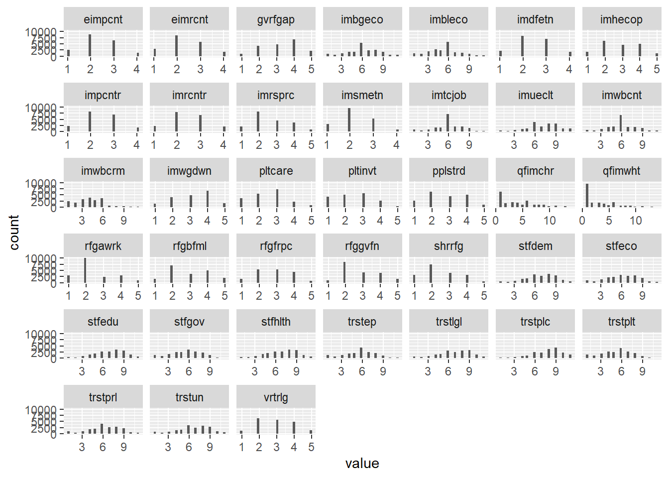

Notice the fact that you can see that the scales are actually categorical (because of the gaps between bars), and that most variables look relatively normally distributed despite being categorical. It’s probably fine to treat them as continuous.

10.0.6 Question 1.f

Check the scale descriptives table again. Are there any incorrectly coded missing value labels, or other inexplicable values?

10.0.7 Question 1.g

The first step in re-analyzing data is replicating the results from the paper by Kestilä. Run a Principal Component Analysis using psych::principal(), and choose the exact same specification as Kestilä concerning estimation method, rotation etc. Do two analyses: one for trust in politics, and one for attitudes towards immigration. Remember that you can view the help file for psych::principal() by running ?psych::principal.

Hint: Use psych::principal()

Click for explanation

10.0.7.1 Trust in politics

Kestilä extracted three components, with VARIMAX rotation. When we print the results, we can hide all factor loadings smaller than the smallest one in their table, to make it easier to read:

library(psych)
pca_trust <- principal(df[, 7:19], nfactors = 3, rotate = "varimax")
print(pca_trust, cut = .3, digits =3)

## Principal Components Analysis
## Call: principal(r = df[, 7:19], nfactors = 3, rotate = "varimax")
## Standardized loadings (pattern matrix) based upon correlation matrix
##           RC3   RC2    RC1    h2    u2  com
## trstlgl 0.779              0.669 0.331 1.21
## trstplc 0.761              0.633 0.367 1.18
## trstun  0.675              0.556 0.444 1.44
## trstep  0.651        0.332 0.549 0.451 1.57
## trstprl 0.569        0.489 0.650 0.350 2.49
## stfhlth       0.745        0.567 0.433 1.04
## stfedu        0.750        0.603 0.397 1.14
## stfeco        0.711  0.300 0.616 0.384 1.44
## stfgov        0.634  0.377 0.587 0.413 1.88
## stfdem  0.369 0.568  0.325 0.564 0.436 2.38
## pltinvt              0.817 0.695 0.305 1.08
## pltcare              0.811 0.695 0.305 1.11
## trstplt 0.510        0.611 0.716 0.284 2.40
## 
##                         RC3   RC2   RC1
## SS loadings           2.942 2.668 2.490
## Proportion Var        0.226 0.205 0.192
## Cumulative Var        0.226 0.432 0.623
## Proportion Explained  0.363 0.329 0.307
## Cumulative Proportion 0.363 0.693 1.000
## 
## Mean item complexity =  1.6
## Test of the hypothesis that 3 components are sufficient.
## 
## The root mean square of the residuals (RMSR) is  0.07 
##  with the empirical chi square  15240.94  with prob <  0 
## 
## Fit based upon off diagonal values = 0.967

For attitude towards immigration, Kestilä extracted five components, with VARIMAX rotation:

library(psych)
pca_att <- principal(df[, 20:44], nfactors = 5, rotate = "varimax")
print(pca_att, cut = .3)

## Principal Components Analysis
## Call: principal(r = df[, 20:44], nfactors = 5, rotate = "varimax")
## Standardized loadings (pattern matrix) based upon correlation matrix
##           RC2   RC1   RC5   RC3   RC4   h2   u2 com
## imsmetn  0.80                         0.72 0.28 1.3
## imdfetn  0.78                         0.79 0.21 1.7
## eimrcnt  0.83                         0.71 0.29 1.1
## eimpcnt  0.80                         0.79 0.21 1.5
## imrcntr  0.83                         0.75 0.25 1.1
## impcntr  0.78                         0.78 0.22 1.6
## qfimchr                    0.82       0.70 0.30 1.1
## qfimwht                    0.76       0.65 0.35 1.3
## imwgdwn                          0.81 0.71 0.29 1.2
## imhecop                          0.75 0.67 0.33 1.4
## imtcjob        0.57              0.34 0.48 0.52 2.0
## imbleco        0.70                   0.55 0.45 1.3
## imbgeco        0.70                   0.60 0.40 1.5
## imueclt        0.57       -0.34       0.54 0.46 2.4
## imwbcnt        0.67                   0.63 0.37 1.9
## imwbcrm        0.66                   0.48 0.52 1.2
## imrsprc              0.61             0.44 0.56 1.3
## pplstrd        0.33       -0.54       0.46 0.54 2.2
## vrtrlg        -0.35        0.46       0.41 0.59 2.8
## shrrfg         0.37 -0.35             0.42 0.58 4.1
## rfgawrk              0.61             0.40 0.60 1.1
## gvrfgap              0.69             0.56 0.44 1.3
## rfgfrpc             -0.39             0.33 0.67 3.3
## rfggvfn              0.58             0.42 0.58 1.5
## rfgbfml              0.60             0.46 0.54 1.6
## 
##                        RC2  RC1  RC5  RC3  RC4
## SS loadings           4.38 3.40 2.78 2.19 1.72
## Proportion Var        0.18 0.14 0.11 0.09 0.07
## Cumulative Var        0.18 0.31 0.42 0.51 0.58
## Proportion Explained  0.30 0.24 0.19 0.15 0.12
## Cumulative Proportion 0.30 0.54 0.73 0.88 1.00
## 
## Mean item complexity =  1.7
## Test of the hypothesis that 5 components are sufficient.
## 
## The root mean square of the residuals (RMSR) is  0.05 
##  with the empirical chi square  29520.06  with prob <  0 
## 
## Fit based upon off diagonal values = 0.98

10.0.8 Question 1.h

Extract the PCA factor scores from the results objects, and add them to the data.frame. Give the PCA scores informative names, based on your interpretation of the factor loadings, so that you understand what they summarize.

Hint: Use $; colnames(); cbind()

Click for explanation

Extracting factor scores

The factor scores are inside of the results objects. Use the $ operator to access them:

head(pca_att$scores)

##           RC2        RC1        RC5         RC3         RC4
## 1   1.9920289  1.3140238 -0.8305392 -0.06329775 -0.08837693
## 4   0.1708174 -1.2167781 -0.4974957 -0.23766146  0.67364069
## 7  -0.3580985  0.3236336 -1.5094405 -0.53052720 -2.20637993
## 14         NA         NA         NA          NA          NA
## 17 -0.1136716 -0.7869911 -1.4664715 -0.07112144  0.41078167
## 20 -0.9188606  2.8264230 -0.3477484 -0.73788338 -1.32089442

We’re going to give these factor scores some informative names, and add them to our data.frame. You should give them different, informative names based on the meaning of the factors!

# Print names
colnames(pca_att$scores)

## [1] "RC2" "RC1" "RC5" "RC3" "RC4"

# Change names
colnames(pca_att$scores) <- c("Att1", "Att2", "Att3", "Att4", "Att5")
colnames(pca_trust$scores) <- c("Trust1", "Trust2", "Trust3")
# Add columns
df <- cbind(df, pca_trust$scores, pca_att$scores)

10.0.9 Question 1.i

Are you able to replicate her results?

Click for explanation

No, probably not. The team of teachers was unable to reproduce this analysis, even though it should be pretty easy to do so…

10.0.10 Question 1.j

Save your syntax and bring your data and syntax to the practical on Thursday.